The Text Inspector
The Text tab in the inspector describes the active document as a whole. This tab has three facets. Overview shows stats for your document, including counts of sentences and words, readability figures, vocabulary, sentence structures, and charts of word class frequencies, grammatical functions, and phrase counts. Details contains the attribute values and tags associated with the document, while Bookmarks shows the passages that you bookmarked in your document.
Statistics describe only the surface of a text. They can help you characterize the document, allow you to choose documents for closer reading, and help you detect anomalies within a dataset (such as transcripts where there never was a break between sentences). However, statistics cannot inform you of what someone intended with the writing, nor can they give insight into why two op-eds differ.
Key terms
When indexing documents, LemmaLoom parses them into their constituent sentences and tokens; tokens refer to individual words and punctuation (see Chapter 21, Analysis and Indexing). Statistics are derived from this division.
- Word refers to any token that is not punctuation or a symbol. Number tokens will also qualify as words.
- LemmaLoom recognizes unique words according to each word’s dictionary form, or lemma; model and models count as one unique word, and so do was and were. These terms are known in linguistics literature as types, giving rise to the term type-token ratio.
- A syllable count represents a rough guess made solely based on the orthography of each word.
- Long words are defined by LemmaLoom as having more than six letters.
- Stopwords are words found in a predetermined list for each language; these refer to commonly used words such as the, of, and is. Words not found in this list are termed content words.
- Shares refer to the proportions expressed as percentages. Given 17 stopwords out of 30 total words, the resulting share will be , shown as 57%.
Opening the Text tab
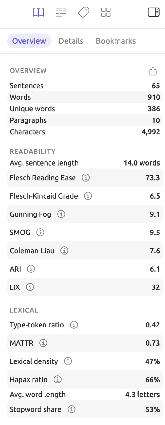
The examples throughout this chapter come from “Climate Debate”, the bundled example project of this guide; you can add the example project to your library with File ▸ Import ▸ Example Project (see The example project in Chapter 1, Introduction). See below for the Text tab of “Running Out of Time”, an activist op-ed with 910 words spread out over 65 sentences.
There is only one column in the Overview facet. It starts from the top and includes five sections of measures (namely Overview, Readability, Lexical, Syntax, and Structure), followed by three bar charts (Parts of speech, Functions, and Phrases). The first section, titled Overview, contains simple counts related to the text, sharing its title with the facet.
To open the Text tab:
- Open a document in the reader.
- If the inspector is hidden, choose View ▸ Toggle Inspector (⌃⌘I).
- Click the book icon at the top of the inspector, or choose View ▸ Inspector ▸ Text (⌥⌘1).
- Click Overview, Details, or Bookmarks in the row of facets below the icons.
By default, your document shows its Text tab and Overview facet until you manually change it. Changes to your tabs and facets are remembered independently by each document whenever you switch document tabs. When viewing documents side-by-side in split view mode, the inspector will show the document in the currently active pane. Click the other pane to inspect the statistics of the other document, although whichever tab and facet had been selected previously will remain intact. Inspectors will remain closed during detail views and when viewing a set; separate inspectors will appear per individual document window.
Statistics need an indexed document in order to display. If indexing isn’t complete yet for the first section of text, then you’ll see the placeholder Statistics become available when indexing completes. The Details facet does what it’s supposed to do regardless of whether or not there are statistics available yet. While indexing occurs, statistics relate strictly to the already processed portion. Document statistics work only with English, German, and Chinese documents; for other languages, the placeholder remains.
The Details facet
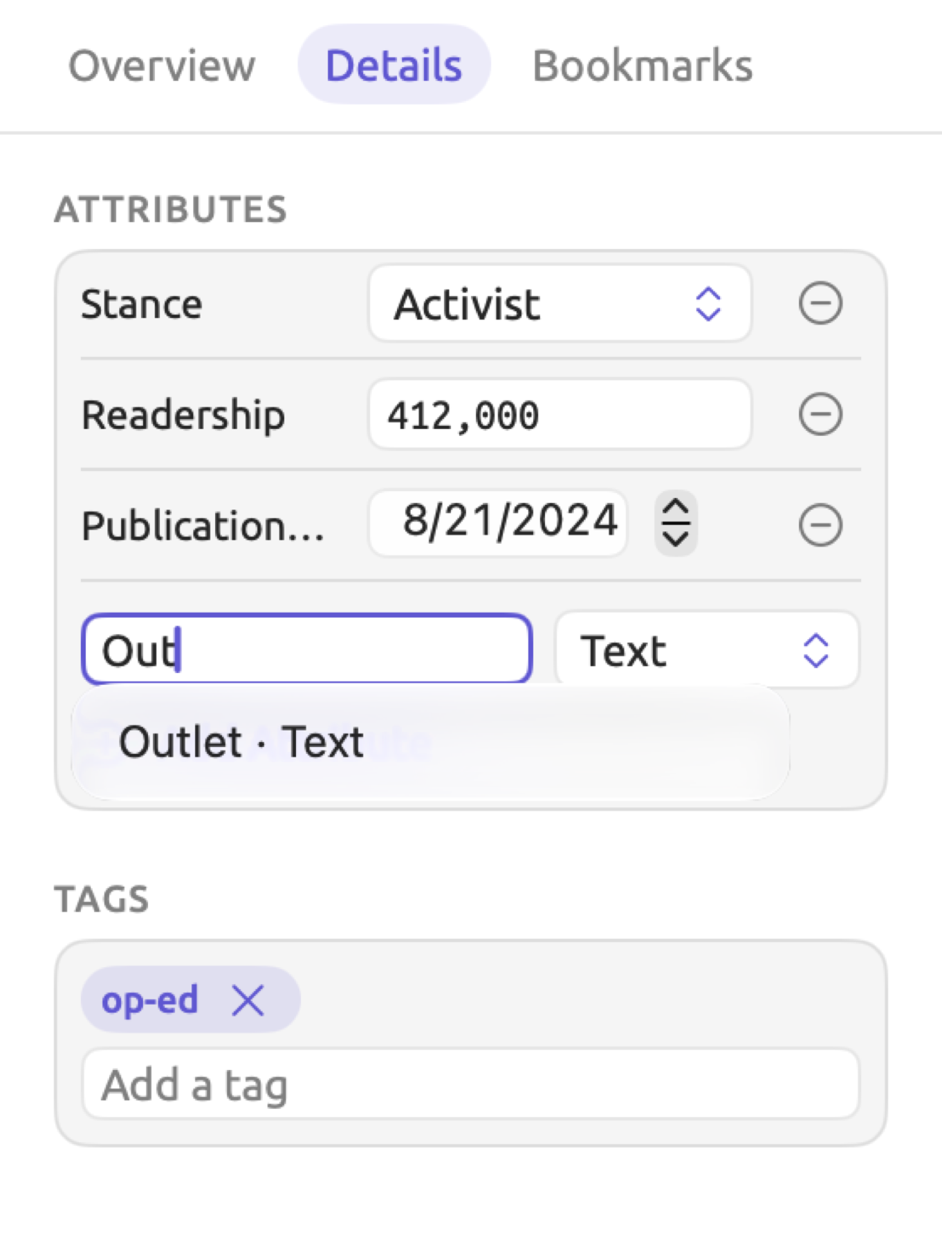
Every document in the “Climate Debate” example project comes with values for four attributes. Values for the “Stance” attribute denote whether the text came from activists, skeptics, or neutral sources. “Readership”, “Publication Date”, and “Outlet” denote the size of the audience, when the article was published, and where, respectively. In the Details facet on the “Running Out of Time” document, Attributes shows “Stance” as “Activist”, “Readership” as 412,000 readers, “Publication Date” as August 21, 2024, and “Outlet” as “The Northern Herald”. Below the Attributes section, under Tags, is the only tag for this document, “op-ed”.
Attributes lists every existing attribute-value pair for the currently active document, providing editing fields for the attributes. It is a place for assigning and modifying attribute values for a single document as you browse through it. For setting attribute values for several documents simultaneously, please see Setting one value for many documents in Chapter 8, Sets, Groups, Tags, and Attributes.
When you need to set a value for an attribute not listed in the current list of attributes for a document:
- Type the attribute’s name in the field below the list. LemmaLoom suggests names already in use in your projects, with their type, as in “Outlet” · Text.
- If the project has no attribute of that name, choose a Type. For a Picker, also type its choices, one per row.
- Click Add Attribute, or press Return.
- Enter the value in the new row.
An attribute is listed only once in each document. If you attempt to add an attribute the document already lists, Add Attribute remains disabled, and its tooltip reads Already added.
When clearing a value, click the remove button at the end of the value’s row (Remove attribute). Tags are inputted via the field that reads Add a tag. Begin typing the desired tag and then press Return, or type a comma after a tag to move to the next one. Suggestions for existing tags appear while typing, and to delete a tag, click the × on it.
All edits happen immediately and affect the document’s translations too. Editing values or tags can both be undone using Edit ▸ Undo Set Value and Edit ▸ Undo Edit Tags (⌘Z); undoing an addition of an entirely new attribute happens via Edit ▸ Undo Add Attribute. For further reading about Entering values and Tagging a document, please refer to Chapter 8, Sets, Groups, Tags, and Attributes.
The statistics at a glance
The list of measurements shown is determined based on the language of your document. The majority of them are common across English, German, and Chinese documents, though the readability formulas are different since most of the formulas were developed with only one language in mind.
| Section | Measure | English | German | Chinese |
|---|---|---|---|---|
| Overview | Sentences, Words, Unique words, Paragraphs, Characters | yes | yes | yes |
| Readability | Avg. sentence length | yes | yes | yes |
| Flesch Reading Ease, Flesch-Kincaid Grade, Gunning Fog, SMOG, Coleman-Liau, ARI | yes | |||
| Flesch-Amstad, Wiener Sachtextformel | yes | |||
| LIX | yes | yes | ||
| Characters per sentence, Avg. word length (in characters), Particle density | yes | |||
| Lexical | Type-token ratio, MATTR, Lexical density, Hapax ratio, Stopword share | yes | yes | yes |
| Avg. word length (in letters) | yes | yes | ||
| Syntax | Mean dependency distance, Avg. tree depth, Clauses per sentence, Embedded clause share, Passive sentences | yes | yes | yes |
| Structure | Dialogue share, Questions and exclamations, Sentences per paragraph | yes | yes | yes |
In the Syntax section, only measures that were provided by the grammar analysis are listed. Where the grammatical structure of a document’s sentences is unknown, this section does not appear.
All values are rounded for presentation purposes. Counts and LIX are whole integers. The Type-token ratio, MATTR, and Mean dependency distance all have two decimal places. The Hapax ratio and shares are expressed as whole percentages. The rest have one decimal place.
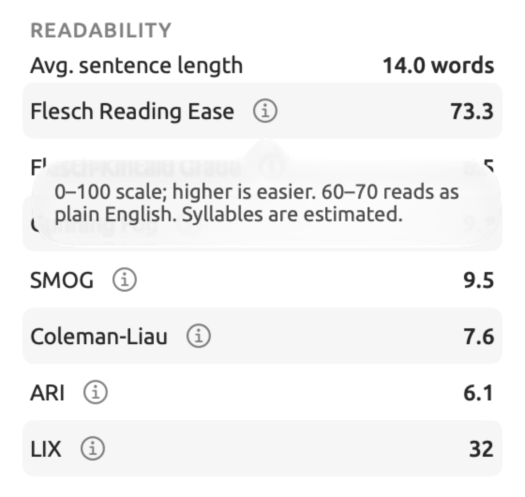
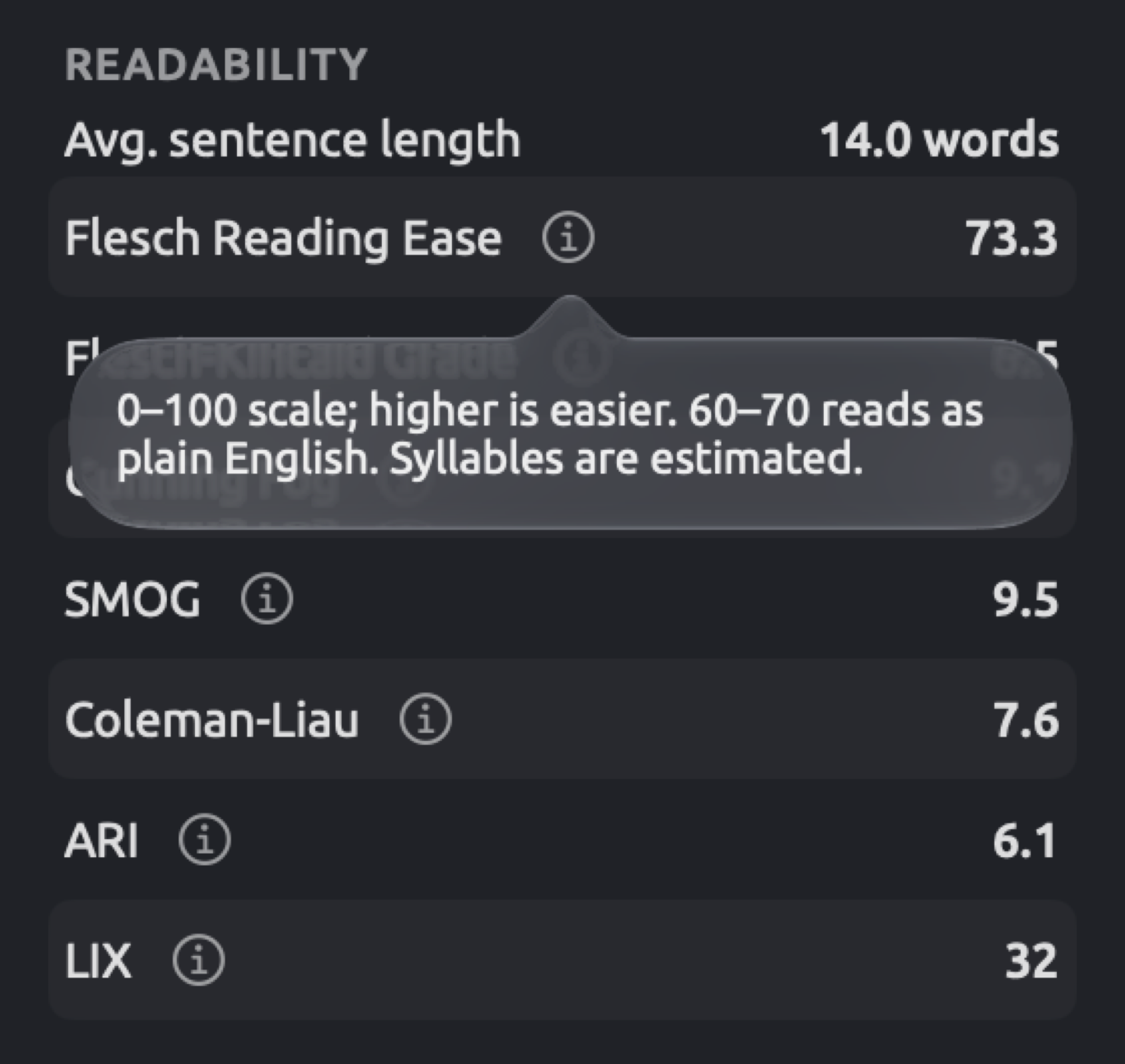
Many measures are accompanied by an ⓘ button next to their name. Click on it for a brief explanation of what the measure represents and the scale in which it operates; clicking elsewhere dismisses it.
Exporting the statistics
To export all statistics in a document to a single file:
- In the Overview facet, find the heading of the Overview section, at the top of the facet.
- Click the export button at the right of the heading (Export as CSV).
- Choose a name and a folder, and click Save. The name suggested is the document’s title followed by
-statistics, as inRunning Out of Time-statistics.csv.
The file has three columns called Section, Measure, and Value, and one row per measure displayed, plus one row per bar of each of the three charts. The value displays the same way as it does in the inspector (rounding and units included), as in 57% or 10.0 words.
There is an export button on the right side of each chart’s heading. This opens a menu containing options for export in PNG and PDF formats (with the chart’s title), and CSV for category counts alone (in Category and Count columns).
The default naming suggestion combines the document and chart titles together, for instance Running Out of Time-Parts of speech.png.
Only one document can be viewed in the inspector at once. In order to consolidate statistical figures of several documents into spreadsheet form for comparative purposes, export each document into a separate file first, and then combine the files, removing the unit symbols and % signs before your calculations.
Finding documents by a statistic
Each measure shown in the table above can function as a rule in a query. A query of this nature allows you to select particular documents that fit the rule, e.g., those that are more difficult to comprehend than plain English, or those containing an exceptionally large proportion of passive sentences.
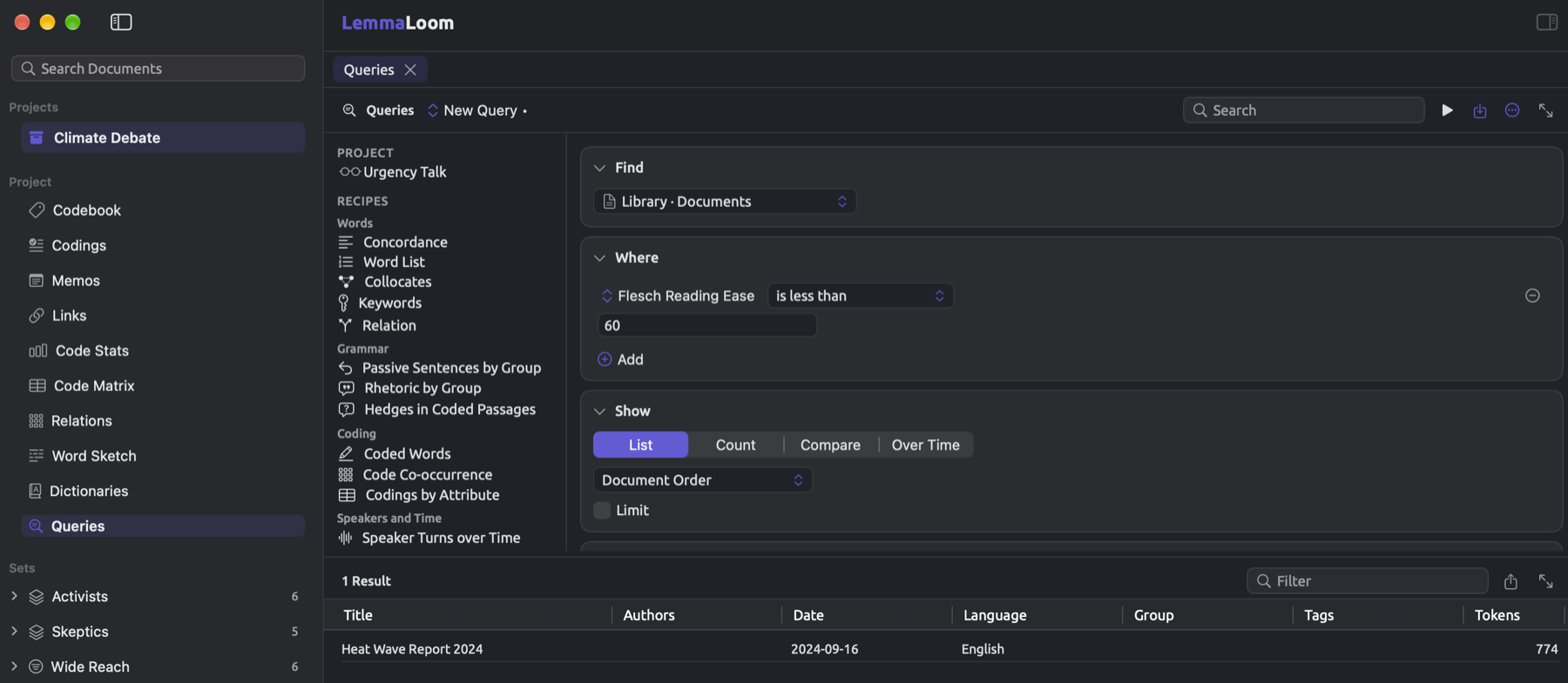
The following image shows a query of this sort within the “Climate Debate” project, seeking documents having a Flesch Reading Ease below 60 (the lower boundary of Flesch’s plain English range), yielding a single document called “Heat Wave Report 2024”.
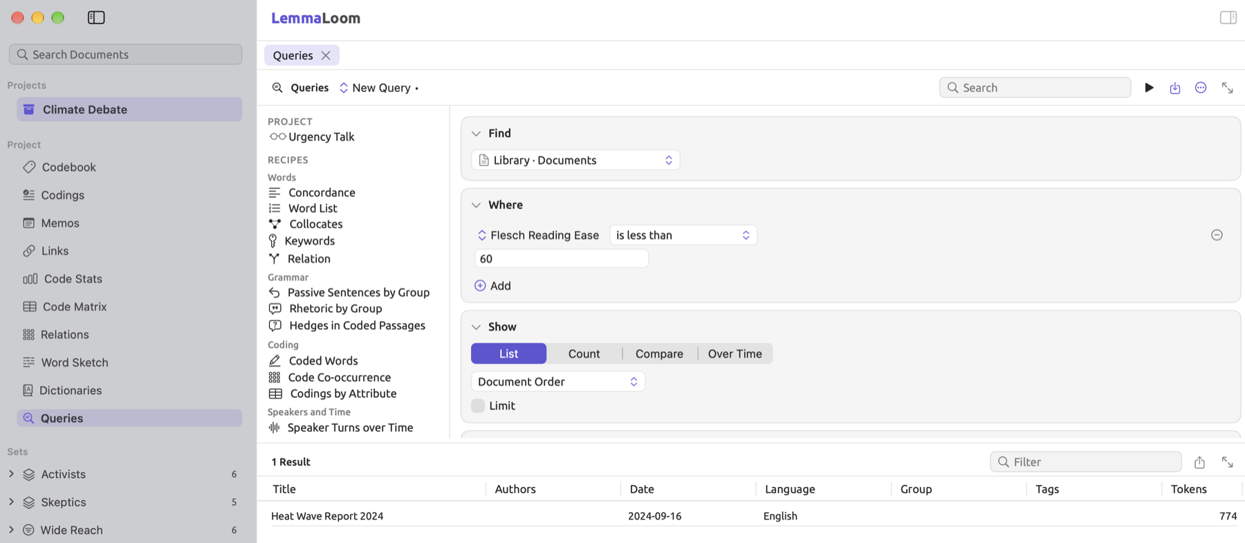
To query documents based on statistics:
- In the navigation sidebar, click Queries under Project.
- In Find, choose Library · Documents.
- In Where, click Add and choose Add Rule.
- Click the field, choose Statistic, and choose the measure, such as Flesch Reading Ease.
- Choose a comparison, such as is less than, and enter the number in Value.
The following are some rules concerning statistic fields in queries:
- The Statistic field is only available in queries made on document sets, projects, and All Projects. While all statistics fields are provided in queries, the only statistic fields in a smart set are Tokens, Sentences, and Characters, which LemmaLoom tracks once a document has been indexed. Tokens counts punctuation marks too; hence, Tokens will be greater than Words. Please refer to Fields in Chapter 15, Building a Query to know where each statistic field is provided.
- The comparison made in a query is against the unrounded number. For example, a score displayed as 86.7 may actually be 86.705; therefore, use comparisons such as is less than, is at least, or is between in place of is.
- Measures shown as percentages, Hapax ratio included, are represented as fractions between 0 and 1 in queries. When searching for documents where the Lexical density is at least 45 percent, the number to input should be
0.45. - A rule skips documents that have no value for its measure. Measures such as Flesch Reading Ease are calculated for English documents only; thus, a rule like is less than
60skips any non-English documents during evaluation. Documents currently being indexed are excluded from the evaluation until their statistics become available.
When the statistics are computed
LemmaLoom calculates statistics on documents and stores them alongside the documents. Statistics on documents are used in the Text tab and the Statistic field in queries, which means that both will always show consistent statistics. Document statistics pertain to the entire document although only annotated sentences may be shown in the reader (see Showing only annotated sentences in Chapter 6, Lenses).
LemmaLoom recalculates the statistics only when changes are made to the document’s text or indexing configuration. Changes include editing and saving the document’s text, altering the document’s language settings, and changing the patterns that exclude text from indexing. Should the statistics not yet be calculated when you visit the Text tab, a spinner icon will appear momentarily until LemmaLoom finishes processing.
Statistics for a translation document, e.g., “Running Out of Time (German)”, will be unique to the translation document and be based on calculations using the measures of its own language.
Counts
The Overview section lists five:
| Measure | What it counts |
|---|---|
| Sentences | Sentences, as indexing divides the text |
| Words | Words, without punctuation and symbols |
| Unique words | Different lemmas among the words |
| Paragraphs | Paragraphs, divided at blank lines or line breaks |
| Characters | Every character of the text, including spaces, line breaks, and punctuation |
Words and unique words
Words refer to indexing tokens without punctuation marks and special characters, according to whatever indexing sees as constituting a token in the language of interest. In English, for instance, indexing splits contractions (don’t = do + n’t), and hyphenated words get split at the hyphen punctuation mark (eighty-four = eighty + four). Since Chinese text contains no word separations in the written form, indexing decides where a word stops and the next starts for counting purposes.
Unique words ignores the capitalization of words, thus making The (capitalized at the beginning of sentences) and the (in the middle of a sentence) equal to each other as a unique word.
Text excluded from indexing, such as timestamps in a transcript, counts only under Characters and, when it forms a paragraph of its own, under Paragraphs (see Text excluded from analysis in Chapter 21, Analysis and Indexing).
Sentences and paragraphs
Sentence boundaries are usually indicated by periods, question marks, and exclamation marks in written texts. In transcripts, sentence boundaries occur anywhere such punctuation is inserted during transcription.
Paragraph breaks are based on the line breaks in your text. If there is a blank line found anywhere in your text, then blank lines function as paragraph breaks, whereas adjacent lines with a line break separating them form a single paragraph. Otherwise, a line break always results in a new paragraph beginning. Blank lines refer to lines containing nothing but whitespace. Transcripts produced by LemmaLoom automatically insert paragraph breaks if there is any change in speaker identity or any pause lasting more than one and a half seconds.
Letters, characters, and syllables
A letter count counts each alphabetic letter in the text, including any Chinese characters. Digits, punctuation marks, and apostrophes do not count toward the letter count measurement. Among all readability formulas, ARI is the only formula that takes into account letters and digits together.
The estimation of syllable count relies on counting consecutive vowel clusters within a word, where vowels include the five letters a, e, i, o, and u, plus the letter y in English and German, and the umlauts ä, ö, and ü in German. Consider heat (ea), again (a and ai), and families (a, i, and ie). When estimating English syllable count, a final e after other vowel clusters is considered silent, except for words ending in le. As a result, words such as wave and were are estimated with one syllable while people has two syllables. Each word must contain at least one syllable; therefore even 2050, which has no vowels, has one syllable.
Words like warned, which is estimated with two syllables due to its -ed suffix, or science, which is estimated as one syllable, not two, are examples of error cases. Words with consecutive a, y, and o vowels such as mayor, estimated at one syllable, are another error case. In German, the word Familien is incorrectly counted with three syllables due to the presence of the cluster ie. Such errors may partly cancel out in practice when calculating overall scores for whole documents.
The example passage
The following sections provide examples. These use a made-up passage similar to what you might encounter in activist literature. The passage below is treated as a complete document.
We were hit by the heat again this summer. So the schools shut for a week and nobody could sleep. The families felt that our mayor had already given up.
Below are its counts:
| Sentence | Words | Syllables | Letters | Long words | Words of 3+ syllables | Words of 1 syllable |
|---|---|---|---|---|---|---|
| We were hit by the heat again this summer. | 9 | 11 | 33 | 0 | 0 | 7 |
| So the schools shut for a week and nobody could sleep. | 11 | 13 | 43 | 1 | 1 | 10 |
| The families felt that our mayor had already given up. | 10 | 15 | 44 | 2 | 2 | 7 |
| Whole passage | 30 | 39 | 120 | 3 | 3 | 24 |
The long words are schools, families, and already. The trisyllabic words are nobody, families, and already. Syllable counts use the estimate of 1 syllable for mayor (which actually has 2 syllables). No digits are used, so the letter count plus digit count comes out to 120. Because the repeats three times, the number of unique words is 28.
Readability
Readability formulas calculate the ease of readability of a text based on just two metrics (sentences’ lengths and words’ lengths), which are relatively straightforward measures to extract objectively from text. Sentence length correlates directly with higher demand on working memory capacity, so longer sentences are harder. The longer words are, the rarer and more abstract they will likely be too. The relationship between the two lengths and the comprehension levels of test subjects (e.g., children at school) was found during studies where test texts were presented to individuals and their comprehension ability assessed. The seemingly bizarre and precise constant factors such as 206.835 come from fitting a mathematical function to these observations.
In a study, you could use readability scores to compare the texts of any media organization to others’, or even assess which side of an argument uses simpler or more complicated linguistic structures than the other.
Grade levels provided by certain formulas describe the necessary schooling years to be able to comprehend the given text adequately without significant effort or confusion. When grades are given without specifying another school system, assume them to belong to the American educational system, where grade 8 equates roughly to age 13 or 14.
Even a sentence composed fully of shorter words can still be hard to understand, and familiar and understandable technical vocabulary still counts by its length in these formulas regardless of the actual understanding of a term.
Notation for readability formula symbols:
| Symbol | Meaning | In the example passage |
|---|---|---|
| Words | 30 | |
| Sentences | 3 | |
| Syllables | 39 | |
| Letters | 120 | |
| Letters and digits | 120 | |
| Words of three or more syllables | 3 | |
| Long words, of more than six letters | 3 | |
| Words of one syllable | 24 |
There are two measures that recur. refers to the mean number of words per sentence; here, = 30 ÷ 3 = 10. represents the mean number of syllables per word; here, = 39 ÷ 30 = 1.3.
Average sentence length
Avg. sentence length is the average number of words per sentence and is calculated by . This measure is provided for all three languages, for instance an average of 10.0 words per sentence for the sample. Most of the scoring metrics introduced below rely on this statistic; hence, it explains a great deal of their behavior. Breaking a long sentence into two makes every score show easier reading.
Flesch Reading Ease
The Flesch Reading Ease, developed by Rudolf Flesch, is a rating system for English texts based on average sentence length and average number of syllables per word in your text. Its values usually fall between 0 and 100, where higher numbers signify easier-to-read texts. The equation looks like this:
, , and are your text’s metrics from the table above. In effect, your starting score is quite high; however, the formula deducts points for having long sentences and words that contain lots of syllables. The syllables weigh far more than sentence length; every additional 0.1 syllables per word in your average costs you around 8.5 points, roughly equal to 8 more words in your average sentence length.
In this example case:
The inspector shows 86.7. Rudolf Flesch described his scores as ranges:
| Score | Description |
|---|---|
| 90–100 | Very easy |
| 80–90 | Easy |
| 70–80 | Fairly easy |
| 60–70 | Standard; plain English |
| 50–60 | Fairly difficult |
| 30–50 | Difficult |
| 0–30 | Very difficult |
The score here is 86.7, meaning that the passage is easy. That is what you’d expect, since the sentences tend to be brief, comprising mostly one-syllable words. The score for “Running Out of Time” (shown earlier in this chapter) is 73.3, meaning it is fairly easy to comprehend. Very long sentences could cause scores less than 0, while very short words could give scores higher than 100.
Flesch-Kincaid Grade
The Flesch-Kincaid Grade index, developed for instructional manuals used by the U.S. Navy, uses the same two metrics as Flesch Reading Ease but converts them into grade levels within the U.S. educational system.
Plugging the numbers in gives:
Rounded up to the nearest tenth, 3.7 corresponds to the grade level where third and fourth graders understand a passage. As both the Flesch-Kincaid Grade formula and Flesch Reading Ease score depend on the same metrics, a high score in one measure typically means a low score in the other.
Gunning Fog
Robert Gunning’s Fog Index tries to measure what educational grade level will be necessary to understand your document based on its sentence length and word difficulty. According to Gunning, hard words include any word which has three or more syllables, excluding compound words whose components were common, names, and any word which reaches three syllables only through suffixes such as -ed.
is the number of hard words; LemmaLoom excludes only names, meaning words that indexing tags as proper nouns, such as Larkhaven. The multiplication factor of 100 turns the ratio of hard words into a percentage.
In the sample passage, there are three hard words (nobody, families, and already), along with no names whatsoever. Calculating this results in:
A Fog Index of 8 suggests around 8 years’ worth of schooling needed, while 12 corresponds to the last year of high school in the United States. Since the second portion of the equation considers exclusively words having three or more syllables, a few such words have considerable influence on the outcome.
SMOG
The SMOG grade (Simple Measure of Gobbledygook) was created by G. Harry McLaughlin. This readability measure involves counting words with three or more syllables, which McLaughlin did within a sample size of 30 sentences. In LemmaLoom, this calculation takes place over the entire document, normalizing the results to 30 sentences.
Here, denotes the number of words of three or more syllables. The square root causes the grade to increase ever more slowly with an increasing number of such words.
For example, the sample passage above has words with three or more syllables in 3 sentences. If scaled up to 30 sentences, that makes for :
The SMOG grade index measures the grade level at which people understand a piece of writing completely. As a result, the number should generally be larger than the Flesch-Kincaid Grade (8.8 vs. 3.7) of the same passage. Words with three or more syllables carry much weight in shorter pieces of writing, leading to the large outcome for this passage.
Coleman-Liau
The Coleman-Liau index differs from the readability indices above because it predicts grades based on letter counts rather than syllable counts. Being computer-friendly was essential to its creation, so instead of estimating the number of syllables, which may produce errors, it counts the exact number of letters.
In the formula, refers to letters per hundred words while refers to sentences per hundred words. More letters per word increase the grade prediction, while more sentences per hundred words (shorter sentences) decrease it.
Consider the example passage, whose 120 letters and 3 sentences make 400 letters and 10 sentences per 100 words:
The predicted grade level falls somewhere between school years four and five.
ARI
Similar to Coleman-Liau, the Automated Readability Index calculates the equivalent American school grade level without syllables, based on characters per word. Characters here consist of letters and digits (variable in the table above).
If and , then:
Since ARI includes digit counts in its calculations whereas Coleman-Liau ignores these, a document containing a lot of digits like “Heat Wave Report 2024” receives a relatively higher grade on ARI compared to Coleman-Liau.
LIX
The Readability Index (Läsbarhetsindex) of Carl-Hugo Björnsson, or LIX for short, is the sum of the average sentence length and the percentage of long words within a passage. This measure is offered for English and German passages. Its mathematical expression is as follows:
In the above formula, is equal to the total number of long words within the passage. With 3 long words out of the 30 words in the example passage:
Its range lies roughly from 20 (very easy) to 60 (very difficult), and 40 (medium difficulty) for the average case. For the example passage, since it is scored as 20, it is considered very easy.
Because LIX measures long words based on letter counts rather than syllable counts, the exact same algorithm applies for calculating LIX regardless of the language. Comparing LIX values across languages, however, is impossible. Partly because German writes compound nouns as one word (like Hitzewelle for heat wave), a German translation of any given text tends to score higher than its English equivalent. As an example, the “Climate Debate” project contains a document called “Running Out of Time”, scoring 32, while its German counterpart is scored as 43. The German version of the example passage (below) has nine long words and scores .
Flesch-Amstad (German)
Toni Amstad extended the Flesch Reading Ease scale to German texts, in which words tend to have a greater number of syllables. Similar to the Flesch Reading Ease formula, results generally range between 0 and 100, wherein larger numbers indicate greater readability.
The German examples use this German adaptation of the excerpt:
Auch in diesem Sommer hat uns die Hitze wieder getroffen. Die Schulen blieben eine Woche zu, und niemand konnte schlafen. Die Familien glaubten, dass unser Bürgermeister schon längst aufgegeben hatte.
| Count | Value |
|---|---|
| Words | 30 |
| Sentences | 3 |
| Syllables | 54 |
| Letters | 166 |
| Words of three or more syllables | 4 (getroffen, Familien, Bürgermeister, aufgegeben) |
| Long words | 9 (getroffen, Schulen, blieben, niemand, schlafen, Familien, glaubten, Bürgermeister, aufgegeben) |
| Words of one syllable | 12 |
The syllable estimate counts Familien as three syllables even though it has four. Now, with :
As per Flesch’s table, whose bands apply here as well, the German version in question is of standard difficulty. Comparing this number with that of the English version from before, 86.7, says nothing about which is easier to read, since the two equations were fitted to different languages.
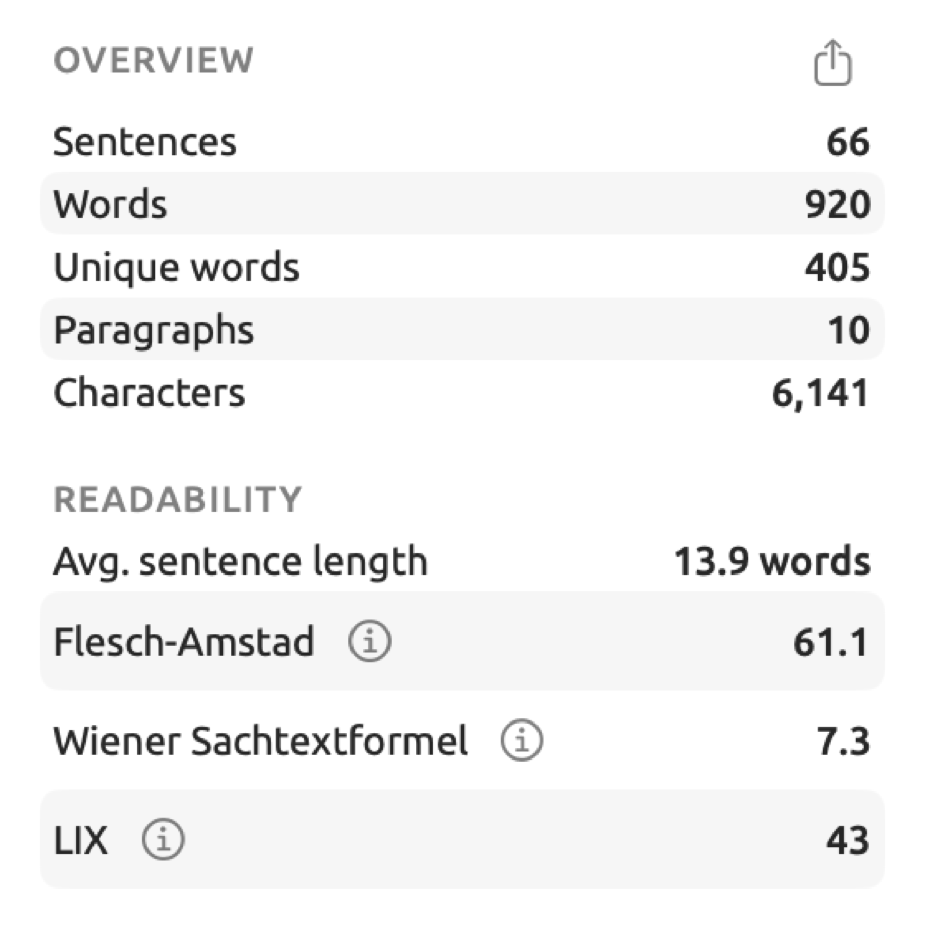
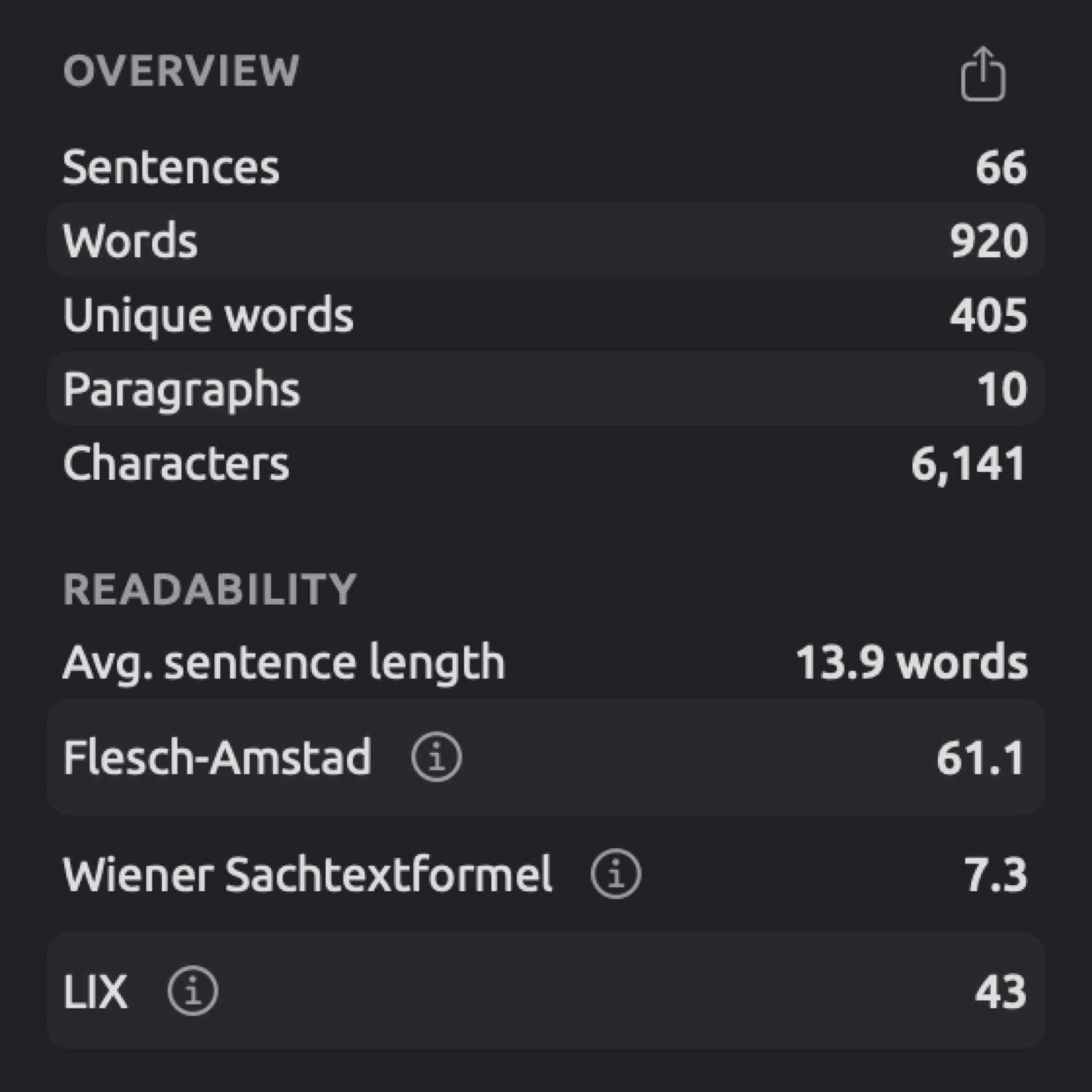
The figure below illustrates the German translation of “Running Out of Time” within the “Climate Debate” project. It has a score of 61.1 in Flesch-Amstad and 7.3 in the Wiener Sachtextformel.
Wiener Sachtextformel (German)
The Wiener Sachtextformel (Vienna formula for non-fiction) was invented by Richard Bamberger and Erich Vanecek for German-language texts. The formula approximates the grade level of a text in the German-speaking education systems, on a scale ranging roughly from 4 (easy) to 15 (very difficult). The version implemented in LemmaLoom is the first of several iterations of the formula, taking into account four measures (the percentage of words of three or more syllables, average sentence length, percentage of long words, and percentage of monosyllabic words) as follows:
For the German-language passage provided above, the percentages calculated according to the order specified by the formula are , , and , respectively. The fourth component is subtracted because many one-syllable words make a text easier. Substituting gives:
This results in:
Thus, rounded to one decimal place, the final score is around 6.0, placing it near the lower end of the scale, so the passage counts as easy.
Chinese measures
The formulas above measure readability in relation to syllables or letters in the case of alphabetic languages. Since the metrics don’t work for Chinese texts, the Readability section of a Chinese document provides three alternatives below Avg. sentence length:
- Characters per sentence measures the ratio between the count of Chinese characters and sentences in your text. Non-Chinese alphabet letters also count here. Furthermore, numbers written in characters will contribute toward character count; for example, 十二 equals two characters. However, numbers written using Arabic numerals such as 12 aren’t considered Chinese characters. As usual, punctuation doesn’t increase character count either.
- Avg. word length is measured in characters. This metric calculates character count divided by word count. Documents containing many two-character words such as 气候 or 邻居 receive higher scores compared to ones where single-character words are common.
- Particle density measures how many particles occur in every hundred words. Particles include words that are annotated with the Particles lens, which are verbal 了, 着, and 过 particles; 的, 地, and 得; and classifiers such as 个 (see Constructions and Particles (Chinese) in Chapter 6, Lenses). Sentence-ending particles such as 吗, 呢, and 吧 aren’t counted.
For these two sentences, indexing splits the words as follows:
我们 / 等 / 了 / 十二 / 个 / 小时 。 邻居 / 也 / 非常 / 担心 。
This results in ten words having sixteen characters distributed within two sentences. Two particles occur, namely 了 and the classifier 个. Thus, Characters per sentence comes to , Avg. word length equals characters, and Particle density reaches particles per hundred words.
The metrics for Chinese don’t map onto any grade levels. Instead, the three serve only to compare one Chinese document with another; on its own, a higher Particle density says nothing about how hard the text is.
Reading the readability scores
Using these formulas on the 30-word example passage in English yields the following results:
| Measure | Score | Kind of scale |
|---|---|---|
| Flesch Reading Ease | 86.7 | Ease, 0 to 100 |
| Flesch-Kincaid Grade | 3.7 | US school grade |
| Gunning Fog | 8.0 | Years of schooling |
| SMOG | 8.8 | US school grade |
| Coleman-Liau | 4.8 | US school grade |
| ARI | 2.4 | US school grade |
| LIX | 20 | Difficulty, about 20 to 60 |
Estimates of schooling for the same excerpt via the five formulas range from 2.4 to 8.8. The difference in numbers comes from the weighting assigned to each feature within a particular formula. This excerpt has several words with three or more syllables in relatively short sentences, leading to high Gunning Fog and SMOG scores but little impact on ARI. The variance among formulas decreases in lengthier documents, but it never disappears entirely. Estimates for the document “Running Out of Time” with the five formulas range from 6.1 to 9.5.
Vocabulary
The Lexical section deals with the words in your document. Through these measures, you get insights regarding whether your document tends to rely heavily on recurring vocabulary or has a varied vocabulary. The type-token ratio, for instance, will inform you about how many unique lemmas were used relative to the total number of words in your text. In it, as in MATTR and the hapax ratio, different forms of a lemma will still be counted as one.
Type-token ratio
The type-token ratio calculates vocabulary diversity as the number of unique words over the total number of words:
Here represents the number of unique words and represents the number of words. If the ratio equals 1, then each word appears exactly once; thus, the fewer times a word repeats itself in the document, the closer to 1 the ratio gets.
The example passage repeats only the, which occurs 3 times altogether, making and the type-token ratio . If a report of 4,000 words had 800 unique words, its ratio would be .
A lower ratio doesn’t necessarily imply a worse vocabulary. The ratio will always fall with longer documents since common words keep repeating and new words occur increasingly less frequently.
MATTR
MATTR, or moving-average type-token ratio, quantifies lexical diversity irrespective of the size of the document. In LemmaLoom, MATTR begins with finding the type-token ratio in a sliding window of the first hundred words of a text, shifting one word along, finding the type-token ratio for words 2 to 101, and so on up until the very end. MATTR is therefore the mean of those ratios.
Here, , , etc. represent the number of unique words found within each window of 100 words sequentially across the document; equals the total number of windows, or, equivalently, the number of words less 99. Dividing each by 100 yields the respective ratio per window; summing and dividing by gives you the mean.
For a smaller-scale illustration, imagine a window of 4 words instead of 100, and consider these eight words, we warn and we wait and we warn. The five windows are thus:
| Window | Unique words | Ratio |
|---|---|---|
| we warn and we | 3 | 0.75 |
| warn and we wait | 4 | 1.00 |
| and we wait and | 3 | 0.75 |
| we wait and we | 3 | 0.75 |
| wait and we warn | 4 | 1.00 |
Here, the mean is . The type-token ratio of the eight words, with 4 unique words, is only .
In a document with 100 words or fewer, the MATTR formula simplifies to being equal to the type-token ratio.
Hapax ratio
The word hapax, Greek for “once”, denotes any word appearing exactly once in your document. The hapax ratio is the proportion of unique words that are hapaxes:
Here is the number of unique words occurring exactly once, while is the number of unique words in total. Sometimes is divided by the number of words instead, which yields a smaller figure. With the example passage, out of the 28 unique words, 27 appear exactly once for a ratio of , shown as 96%. In the hypothetical 4,000-word document containing 800 unique words with 400 hapaxes, the ratio would equal 50%.
A high hapax ratio tends to show that many words appear in passing, including proper nouns. As is the case with the type-token ratio, the hapax ratio depends upon length; with a short document most words occur exactly once.
Lexical density and stopword share
Stopword share is the proportion of words in a document that are in the list of stopwords for that document’s language. Conversely, Lexical density is the proportion of words in a document that are not stopwords; thus, both proportions add up to 100 percent.
Consider the example passage, for instance, which consists of thirty words. There are seventeen stopwords here, namely we, were, by, the, again, and this in the first sentence; so, the, for, a, and, and could in the second; and the, that, our, had, and up in the third. The stopword share of this passage would then be , whereas the lexical density is .
Natural speech tends to have less lexical density than edited writing does, due to pronouns and auxiliaries. Finding that the stopword proportion in a transcription is low compared to natural speech can be a sign that the transcript was summarized rather than transcribed word for word.
Lists of stopwords come built in, and they are fixed per language:
- The list of English stopwords contains around 160 words including articles, pronouns, prepositions, and conjunctions; conjugations of be, have, and do; modal verbs like can, should, must, and the rest; negative not and no; and common adverbs like very, also, and again.
- The list of German stopwords contains roughly 210 words, including, besides articles, pronouns, prepositions, and auxiliaries, the modal particles ja, doch, mal, eben, and halt.
- The list of Chinese stopwords contains about 150 words, among them 的, 了, and 是; pronouns; 不 and 没有; and common prepositions and adverbs.
A word qualifies as a stopword if it matches the list in terms of its lemma or token form. Content words that can appear to be function words include nobody in the example passage. The query field Stopword uses the same lists.
Average word length
Avg. word length in the Lexical section is the ratio of letters to words, , represented in letters. The example passage has letters per word, while the German translation has . Since numbers contain no letters, texts with lots of numbers will have a slightly lower Avg. word length than those that don’t. In the case of Chinese texts, the metric appears under Readability, expressed in characters.
Syntax
The Syntax section analyzes your sentences for how they are constructed beyond measuring sentence lengths. Measures include looking into the distance between words related to each other, nesting of clauses inside other clauses, and other similar measures that reveal the complexity of the sentence structure. They rely upon two parts of the grammar analysis.
The dependency analysis refers to analyzing the relationship between words within a sentence in terms of the head word on which each word depends. In a fair share, for instance, fair and a depend upon share. Each sentence has one root word, which does not depend upon any word (generally the main verb in a sentence). The links between words and their heads are displayed graphically via the inspector under the Grammar tab (see Chapter 11, The Grammar Inspector).
The phrase analysis groups the words of a sentence into phrases and clauses nested inside one another.
Mean dependency distance
Dependency distance measures the distance between a word and its head measured in terms of positions in the sentence. Mean dependency distance is calculated by taking the average of dependency distances for every word within a document having a head:
Here, to refer to individual dependency distances, while denotes the number of words having heads, that is, every word except the root of each sentence. Punctuation occupies positions, yet does not contribute toward the total dependency distances.
The word pay functions as the root verb in the sentence The richest countries rarely pay a fair share. Word numbers indicate positional order, beginning with 1. Words along with their heads appear below:
| Word | Position | Head | Head’s position | Distance |
|---|---|---|---|---|
| The | 1 | countries | 3 | 2 |
| richest | 2 | countries | 3 | 1 |
| countries | 3 | pay | 5 | 2 |
| rarely | 4 | pay | 5 | 1 |
| a | 6 | share | 8 | 2 |
| fair | 7 | share | 8 | 1 |
| share | 8 | pay | 5 | 3 |
The sum total of these 7 dependency distances is 12. Thus, the mean dependency distance of this sentence is . Dependency distances are high when there is significant separation between the related words. In research on sentence processing, higher dependency distances correlate with increased processing done by the reader. Lengthier sentences, embedded clauses, and verb-final construction of German clauses contribute to higher scores here. Mean dependency distance has no universal scale; it only holds significance when compared with other documents in the same language.
Average tree depth
For every word, the path upwards through its heads to the hierarchy’s root defines its depth. The number of hops needed is equivalent to the depth of the word. Depth for a sentence is calculated by finding the highest depth value among all of its words. Avg. tree depth is merely the average depth of sentences in a document.
In the sentence above, the words countries, rarely, and share link directly to the root, meaning they only take 1 hop (depth = 1). The words the, richest, a, and fair all need 2 hops before reaching the root; therefore, the depth of this sentence is 2. For instance, consider another document containing sentences with depths of 2, 4, and 6. Then the average tree depth is .
Clauses per sentence and embedded clauses
Clauses per sentence calculates how many clauses, according to the phrase analysis, occur per sentence on average. This measure calculates , where is the total number of clauses in your document, while is the total number of sentences in your document. Embedded clause share calculates what share of your document’s clauses are not main clauses. Every sentence with at least one clause is considered to have exactly one main clause. As such, this measure divides by , where is the number of sentences having at least one clause. The combination of these measures allows you to gauge the degree to which a writer embeds one idea within another rather than setting them side by side.
Formally, Clauses per sentence is , while Embedded clause share is
The count follows the phrase analysis closely. For instance, an English subordinate clause because the heat was dangerous counts as two layers. It includes its inner clause the heat was dangerous. As a consequence, the sentence We stayed inside because the heat was dangerous. has three clauses in total (the whole sentence, the because clause, and the clause inside it). On the other hand, the sentence Nobody complained. has just one. Consider the calculation for a document consisting of those two sentences:
- Clauses per sentence equals .
- Embedded clause share equals , or 50%.
Because of the layering, the values come out higher than a school grammar’s count of clauses.
Passive sentences
Passive sentences refers to the proportion of sentences within your document that have one or more occurrences of passive constructions. Multiple occurrences of passives in a single sentence will not change the count. For instance, in a document with 40 sentences in total, and six of those having passives, the proportion becomes .
What counts as a passive depends on the language:
- In English, the grammar analysis detects the subject and auxiliary verb in a passive sentence; one example is this from “Heat Wave Report 2024”, This report was prepared by the agency’s climate monitoring service.
- For Chinese, any occurrence of a sentence with 被 and other recognized passive constructions will be included, as with the 被 passive aspect of the Constructions lens.
- In German, a passive with werden and a past participle counts whether or not the agent is named, as in Dieser Bericht wurde erstellt and Dieser Bericht wurde von der Klimaüberwachung des Amtes erstellt. A passive with sein counts only when a von or durch phrase names the agent, as with the Passive voice device of the Rhetoric lens.
Occasionally, passives omit information on who performed an action. In “Heat Wave Report 2024”, for instance, responsibility for checking on older people living alone was not clearly assigned.
Structure
The Structure section contains three metrics.
Dialogue share calculates what percentage of words occur between double quotation marks. Consider, for instance, the artificial sentence My neighbor always said, “Our summers are mild.” Four out of eight words occur in quotations here, making a dialogue share of 50%. In news reports, such as “Carbon Tax Debate”, quotation marks are used to highlight direct quotations from speakers, and the share shows how much of the text overall is other people’s words. LemmaLoom pairs the quotation marks to estimate the share:
- Straight quotation marks (
") open and close sequentially. - Curly quotation marks open with “ and close with ”. In German documents, „ opens and “ closes.
- « and the Chinese corner brackets 「 and 『 open, and », 」, and 』 close. In German documents, » opens and « closes.
- Single quotation marks are ignored.
An unpaired quotation mark causes all subsequent words to count as quoted. A surprisingly high value often suggests there may be a rogue quotation mark somewhere in the document.
Questions and exclamations calculates the percentage of sentences ending with a question mark or an exclamation mark. It includes the full-width characters in Chinese texts. Note that only sentences whose final token is either an exclamation or question mark qualify; sentences ending with a closing quotation mark after the question mark are excluded. In a document containing 80 sentences, among which there are 18 questions and 2 exclamations, Questions and exclamations amounts to . A high value in opinion pieces and speeches may suggest the presence of rhetorical questions, such as the one bookmarked in “Running Out of Time”. As usual, the statistics pertain to the document’s entirety, including the host’s questions in a transcript such as “Radio Debate”.
Finally, Sentences per paragraph is obtained by dividing the total number of sentences by the number of paragraphs. For example, 120 sentences spread over 40 paragraphs produce a ratio of 3.0 sentences per paragraph. Transcription with LemmaLoom produces transcripts with paragraphs ending at every change of speaker and at substantial pauses; hence, the metric provides a rough idea of how many sentences speakers utter continuously.
Parts of speech, functions, and phrases
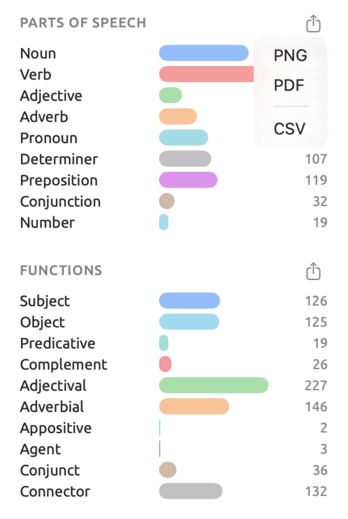
Below the measures, three bar charts show word and phrase distribution across categories in your selected document. Each row includes the category name, a bar, and a number that represents how many times the category was used in the selected document. Note that these statistics do not contain unused categories; the bars use the standard colors of the matching lens, even when other colors were chosen in the Lenses pane of Settings.
- Parts of speech shows word count statistics in the ten classes of the Word class lens from Noun to Interjection (see Word class in Chapter 6, Lenses). Note that all other types of words, including foreign words, are excluded from this statistic.
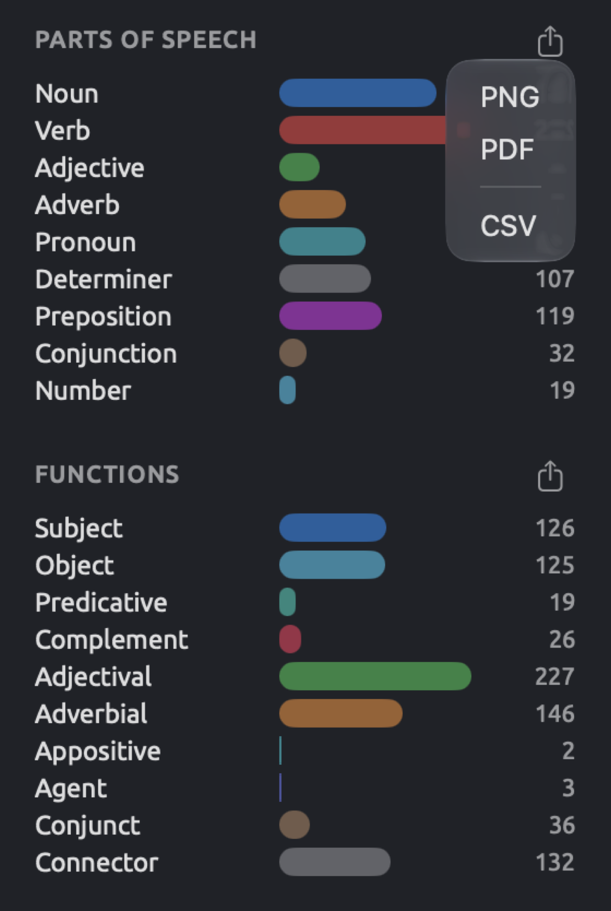
- Functions represents word count statistics in each of the ten functions in the Grammatical function lens, ranging from Subject to Connector (see Grammatical function in Chapter 6, Lenses). Note that the root words without a function (typically the main verb) in each sentence are ignored, as well as words where the relationship does not fit into the ten types of grammatical functions, so these statistics’ totals will be lower than the total number of words in the document.
- Phrases shows the phrase count for each kind of phrase in the Phrase lens from Noun phrase to Interjection (see Phrase in Chapter 6, Lenses). Note that nested phrases each count, e.g., in our valley would count as a prepositional phrase and our valley would be counted once more in the noun phrase category, while clauses are tracked separately under Syntax.
In the “Climate Debate” sample project, “Heat Wave Report 2024” is heavily focused on nouns and prepositions but uses very few pronouns compared to the op-eds or “Radio Debate”. The figure below illustrates the Parts of speech and Functions charts of the “Running Out of Time” document.
To see what words comprise each bar, turn on the matching lens in the reader.
The Bookmarks facet
The Bookmarks facet displays the document’s bookmarks ordered by position in the document. In “Climate Debate”, for instance, “Running Out of Time” has 1 bookmark located in its final paragraph, specifically at the question What exactly are we waiting for? with the comment “Rhetorical question at the turn to the closing appeal”. The heading displays how many bookmarks are associated with the document, which is why the heading is Bookmarks (1) in this case. For instructions on bookmarking, refer to Bookmarks in Chapter 7, Coding.
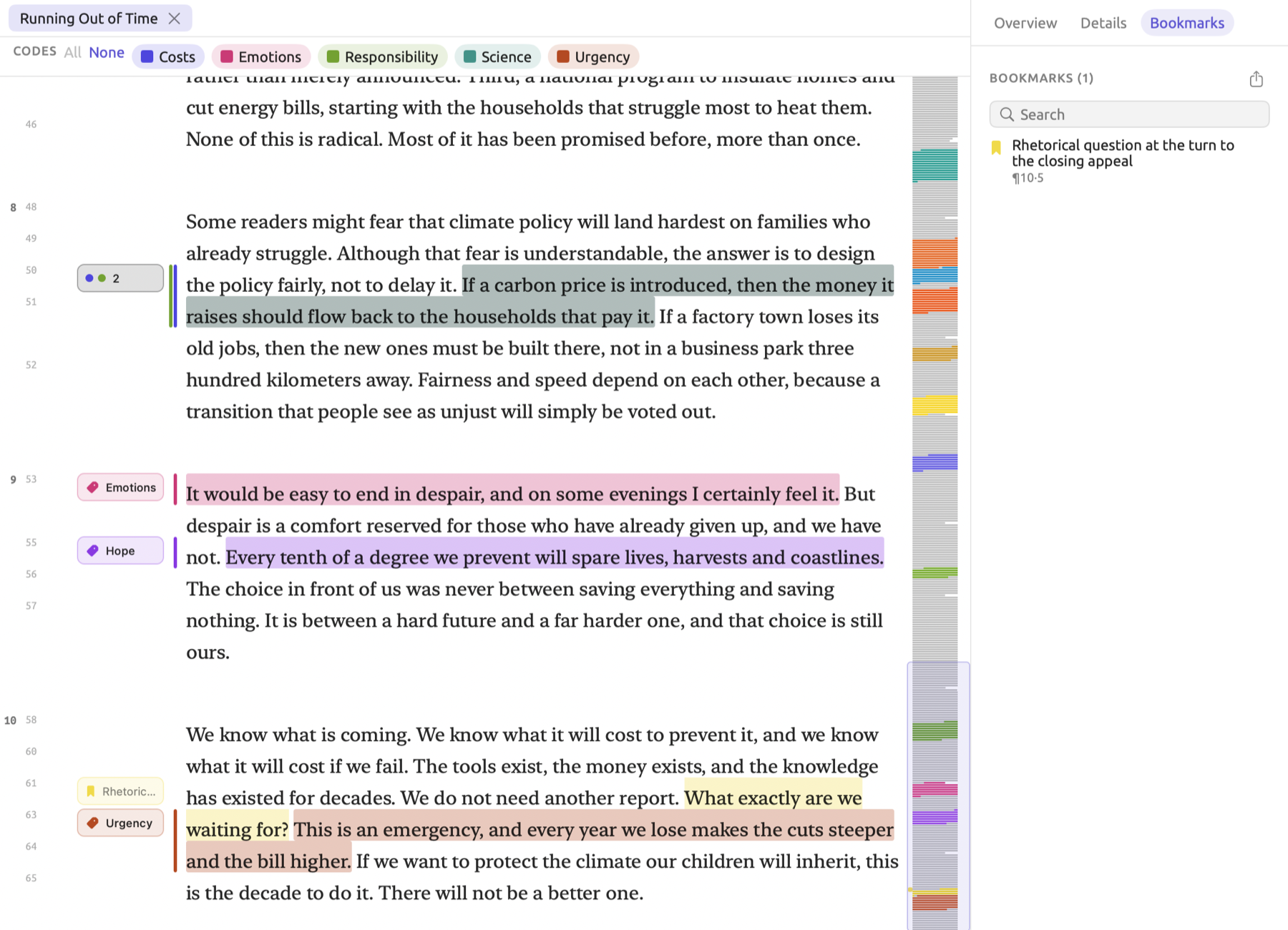
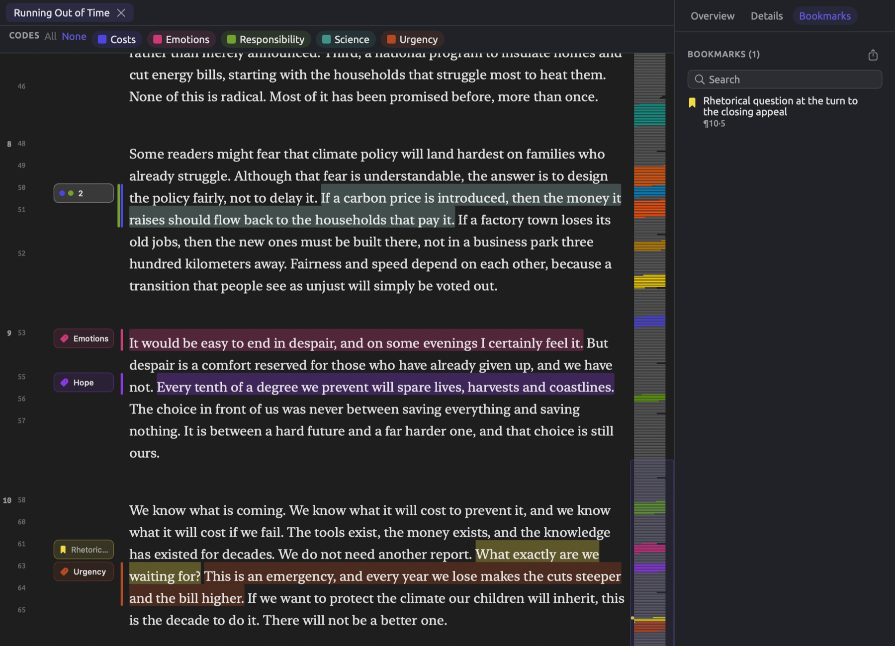
Each row lists:
- a bookmark icon in the color of the bookmark, or gray if it has No color;
- the comment of the bookmark, or, if there isn’t a comment, the bookmarked text itself up to three lines long;
- and the location of the bookmark, like ¶10·5 for the fifth sentence of the tenth paragraph. Hovering the mouse pointer over this location will reveal it in full, as in Paragraph 10, sentence 5.
Clicking on a row navigates to the bookmark. Should only annotated sentences appear in the reader and not the selected bookmark, everything else in the document gets displayed before navigating to the bookmark.
Above the list is the Search field. Typing anything in this field filters the list to the bookmarks whose comments or text contain what you typed; case sensitivity doesn’t play a role here. Nonetheless, the number in the heading counts all the bookmarks regardless of this action.
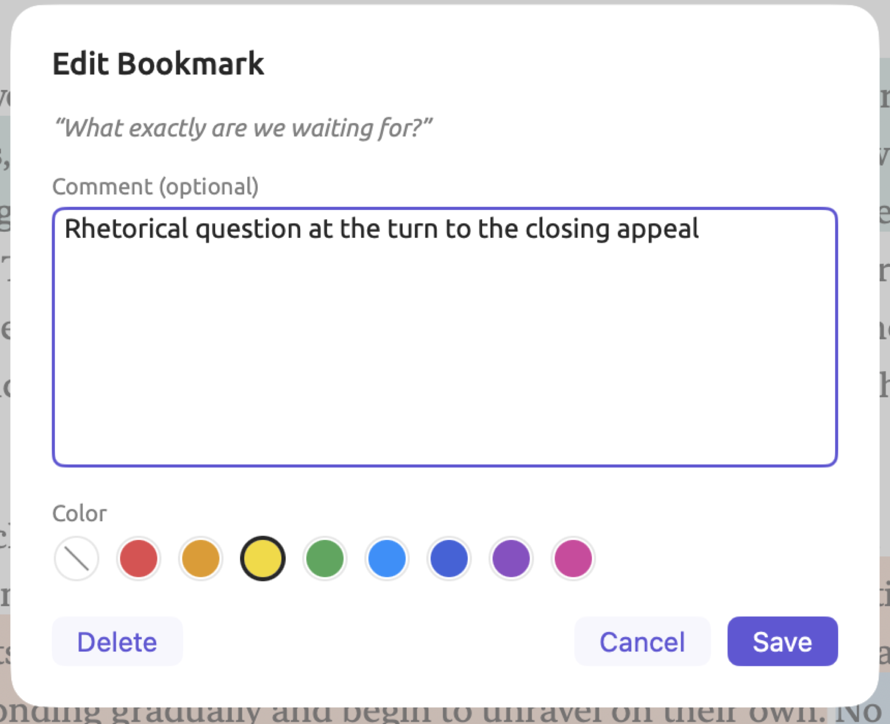
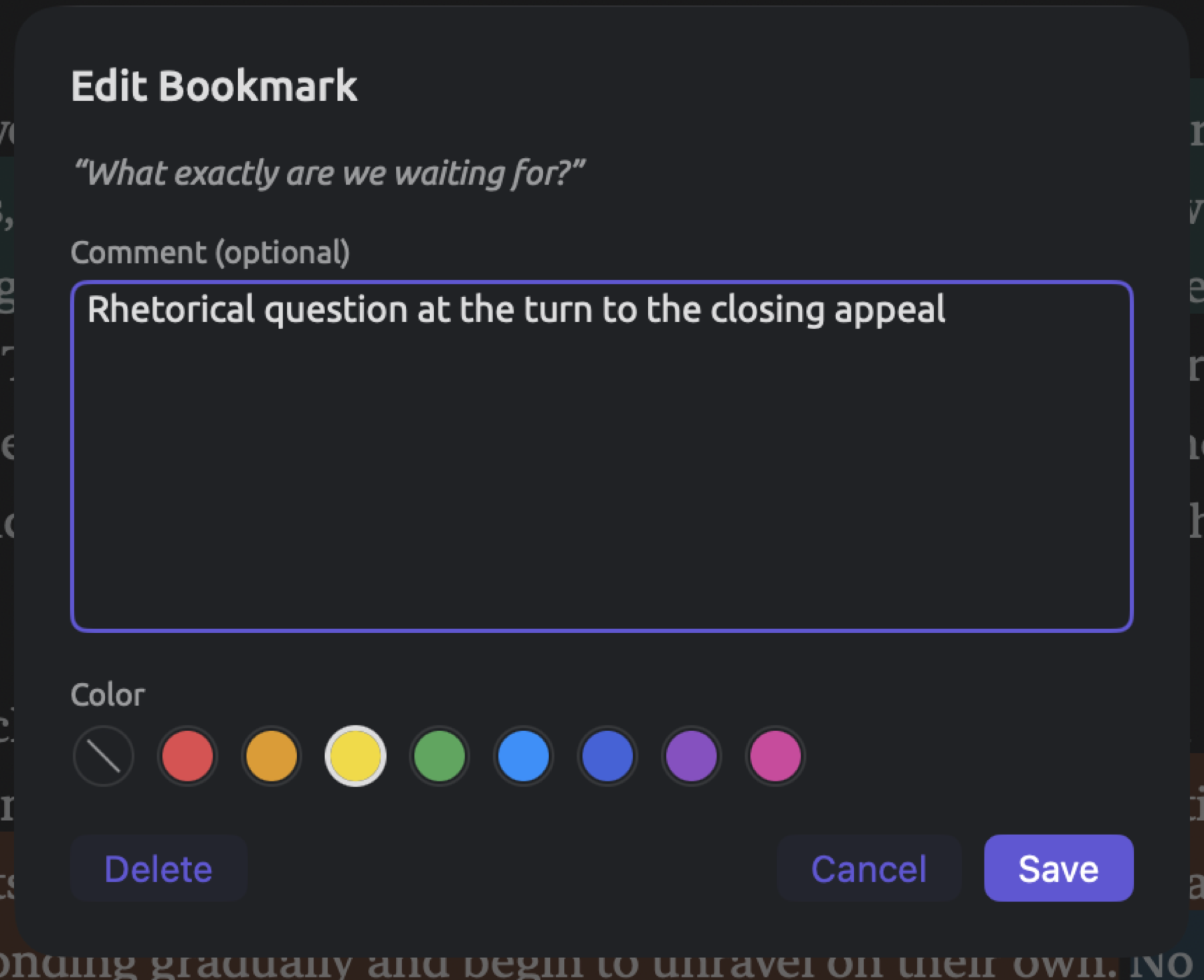
To change a bookmark’s comment or color:
- Right-click its row and choose Edit.
- In the Edit Bookmark dialog, which shows the bookmarked passage, change Comment (optional) or Color.
- Click Save.
To remove a bookmark, right-click the row associated with it and select Delete. Alternatively, click Delete at the bottom of the Edit Bookmark dialog. Your changes are immediate; use Edit ▸ Undo Remove Bookmark (⌘Z) to restore a deleted bookmark. Edit ▸ Undo Edit Bookmark (⌘Z) will undo an edit action performed on a bookmark.
If there were translations available for the document where you marked a bookmark, then that bookmark exists in every translation. It is linked to the matching passage in each translation; edits and deletions of bookmarks happen across all of them. When creating bookmarks based on hits in a query (Bookmark Hits…), the resulting bookmarks will show up here just as regular bookmarks do (see Bookmark Hits in Chapter 18, Using Query Results).
Bookmarks can be exported by clicking the export button at the right of the heading (Export as CSV). The exported file includes three columns (Location, Text, and Comment) containing all of the bookmarks currently listed, which means that only matched bookmarks would be included following a search operation. The filename suggestion is the document’s title followed by -bookmarks.