Sketch Space
Word sketches illustrate grammatical behaviors of a word in a document, set, or project. However, Sketch Space takes the sketch of a word further by splitting its relations by the codes that cover each occurrence, or, in a set or project, by the values of an attribute, like “Stance” or “Readership”.
A word sketch shows a word’s partners across the entirety of your document, set, or project. Sketch Space considers how those partnerships vary depending upon their context. It shows whether this word has a different set of partners when used in passages coded “Science” vs. “Urgency”, and whether the activists use the same partners with the word as the skeptics. As a general rule, you discover a word within its word sketch before exploring Sketch Space, once you have codes or attributes whose differences you want to look into. Comparisons of codes require sufficient amounts of materials to have been coded; otherwise, almost all occurrences are going to fall under the category Uncoded, giving you nothing to compare.
Consider the word climate in the texts of “Climate Debate”. In passages coded “Science”, writers predominantly pair climate with research as seen in climate science or climate model (“Every climate model contains processes too small or too fast to simulate directly”). Conversely, an occurrence of climate in a passage coded “Urgency” portrays the climate acting (“Meanwhile the climate has not waited for us”). Sketch Space displays those differences alongside one another with columns representing the codes and each row showing a specific grammatical relation, while providing the sentences behind every counted number.
Further explanations concerning word sketches, including grammatical relations and the logDice score, can be found in Chapter 12, Word Sketch. Information about coding is covered in Chapter 7, Coding. All examples used in this chapter are drawn from “Climate Debate”, a sample project available via File ▸ Import ▸ Example Project (refer to The example project within Chapter 1, Introduction).
Key terms
- The center word is the word being compared. Sketch Space works with dictionary forms, or lemmas; hence, scientists and scientist will be regarded as the same word.
- Each column represents one of several things, either a code, or the value of an attribute, or Uncoded. The columns capture occurrences of the center word in passages with codes, and in documents with values of attributes. Occurrences of the center word in passages with multiple codes are duplicated accordingly, while occurrences which fall outside any of the codes are collected in the Uncoded column.
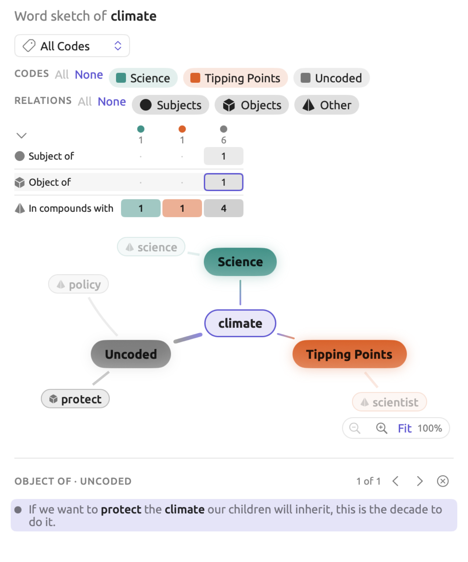
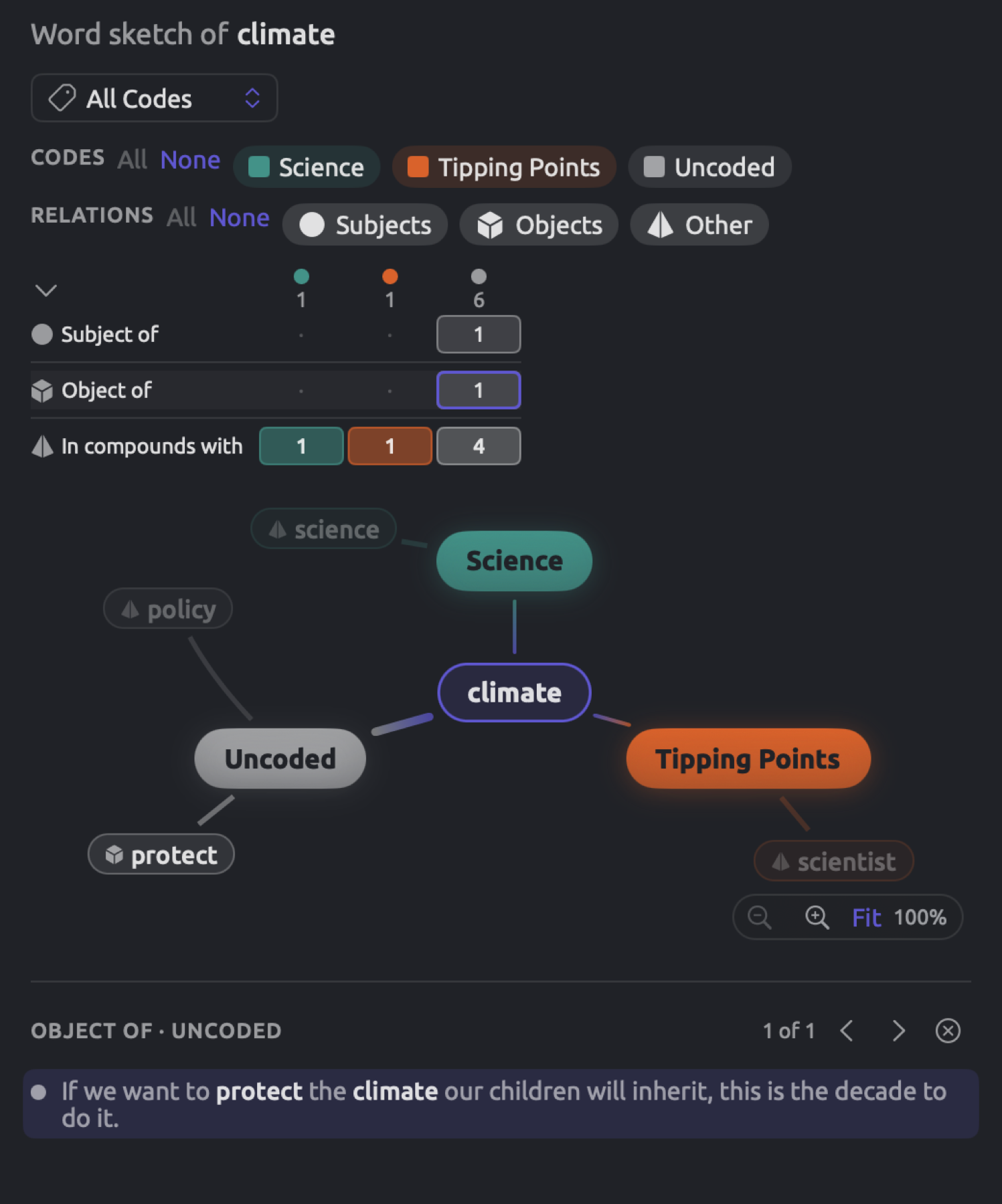
- Relation refers to any grammatical connection between the center word and another word. In the sentence “If we want to protect the climate our children will inherit”, climate functions as the object of the action protect. Therefore, this example contributes one relation to the Object of row.
- Partner denotes the other word involved in the relation. Partners are ranked according to logDice, a score for how firmly a partner belongs with the center word.
- Sectors refer to the five categories into which relations fit (Subjects, Objects, Modifiers, Prepositional phrases, and Other). You use sectors as filters in Sketch Space.
- Hub is the term used to refer to a column when placed in a comparison map.
- Evidence lists store sentences associated with counts, partners, and hubs.
- Characteristic relations are relations employed by a column clearly more often than by the rest of the material. Grids annotate counts of characteristic relations with an asterisk.
logDice compares pairs based on their frequencies, divided by the frequency of their partner words together with the overall frequency of the center word involved in the relation. logDice has a maximum value of 14 points; each point lower means the pair makes up half as large a share of the two words’ use. For the full calculation, see logDice in Chapter 12, Word Sketch.
Where Sketch Space is
Sketch Space can be found in two places; each instance has the same interface:
- For a single document, it’s in the inspector’s Multimode tab, where codes are the columns.
- For a set, tag, or a full project, Sketch Space is accessed via the Multimode mode of the Word Sketch view and Word Sketch window, wherein codes and attribute values are the column options. Sketch Space for sets and projects has more details about those.
When reading and coding a document, you’ll use the inspector because it tracks the currently selected word in the reader. However, since a document usually contains insufficient occurrences to get a *, it’s recommended to use either a set or project for reliable comparison results.
Documents must always be indexed first in order to use Sketch Space, but LemmaLoom will automatically index documents written in English, German, and Chinese. For unindexed documents, the inspector displays Grammar becomes available when indexing completes until indexing is done. More info regarding indexing can be found in Chapter 21, Analysis and Indexing.
Comparing a word across codes
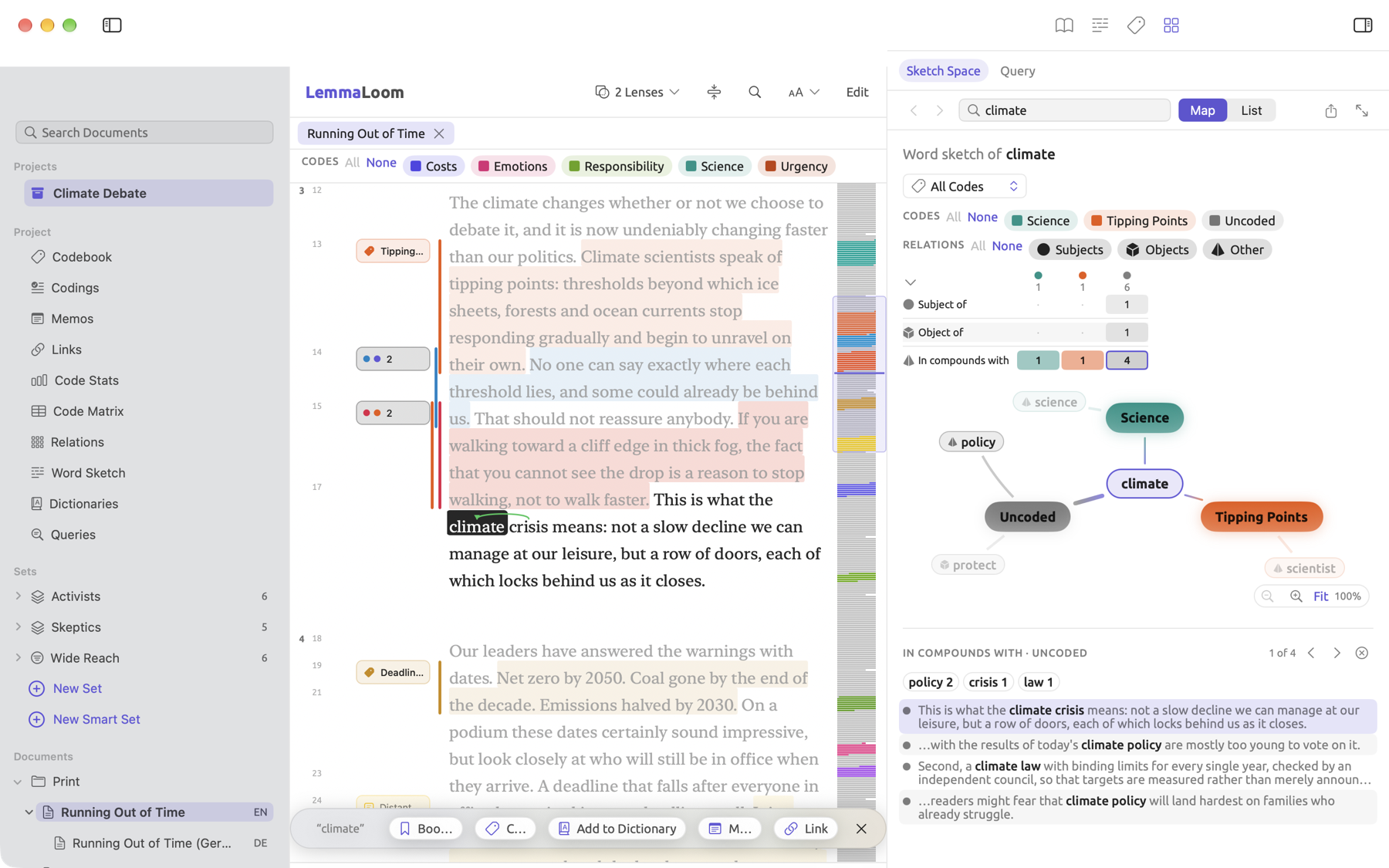
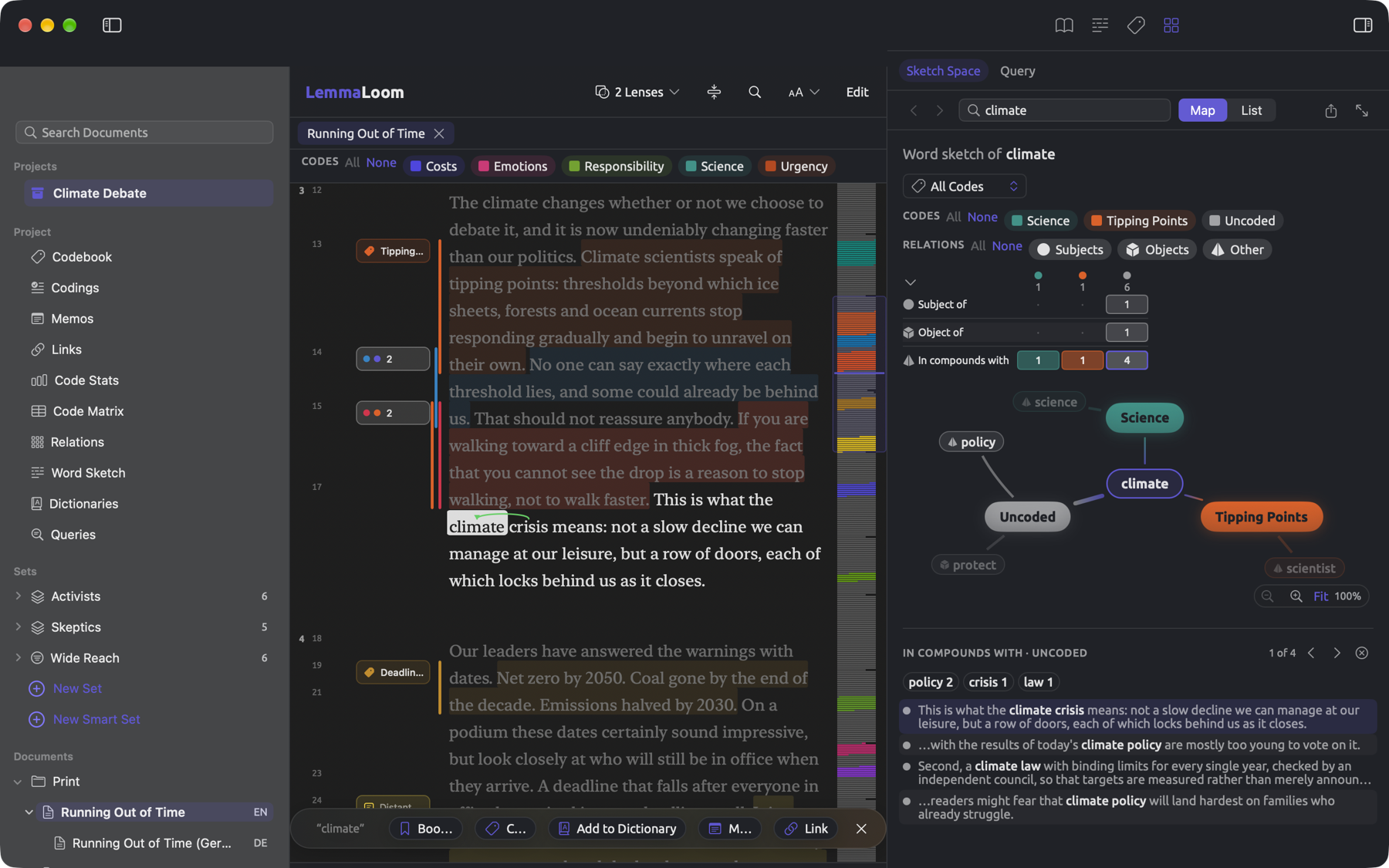
“Running Out of Time”, an op-ed authored by activists in “Climate Debate”, uses the word climate eight times. One instance is within a passage coded “Science”, another within a passage coded “Tipping Points”, a subcode of “Urgency”, and the remaining six instances are uncoded. Sketch Space displays these occurrences as three columns, allowing you to examine the distribution and usage of climate within each code or elsewhere in the text.
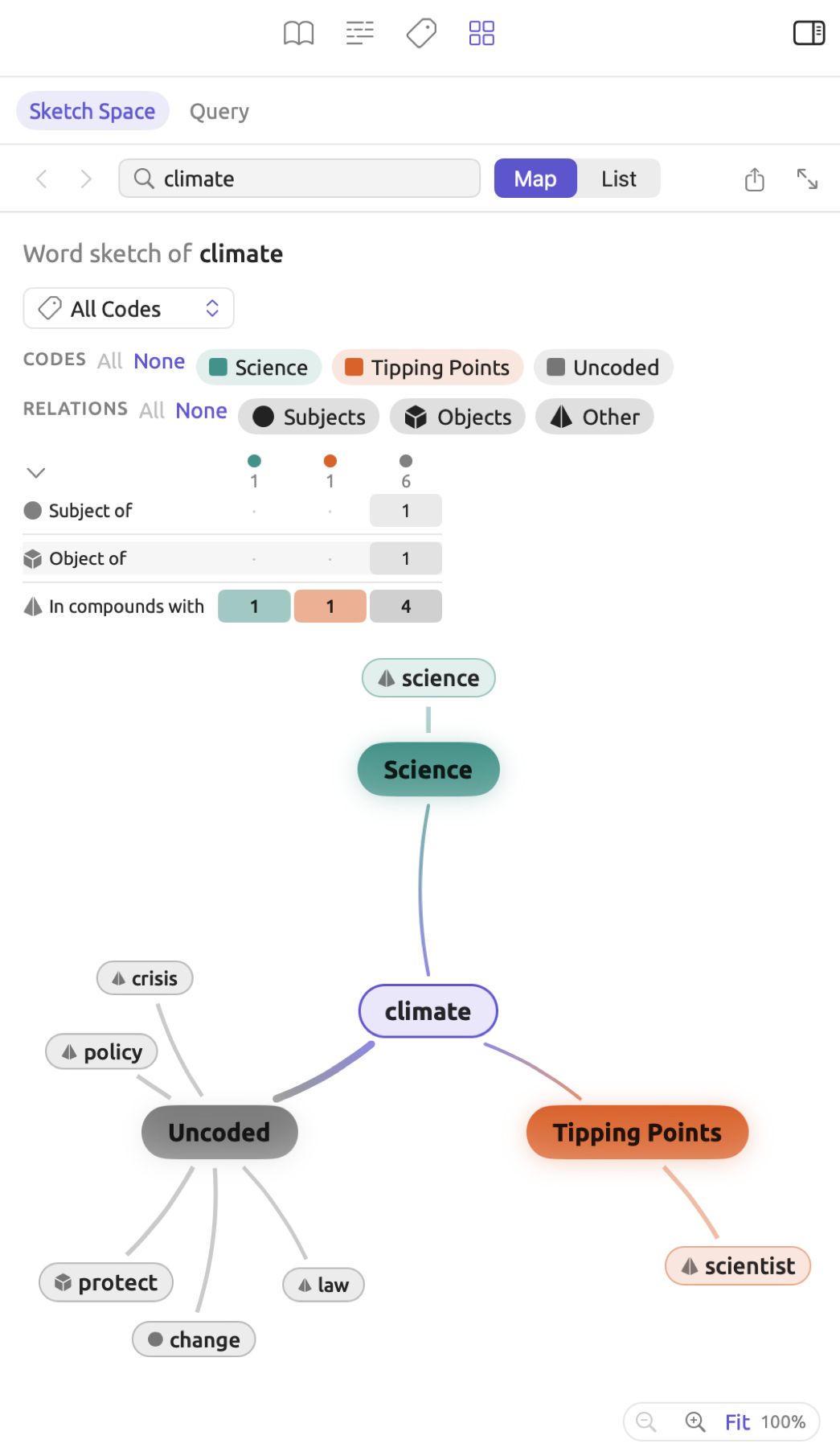
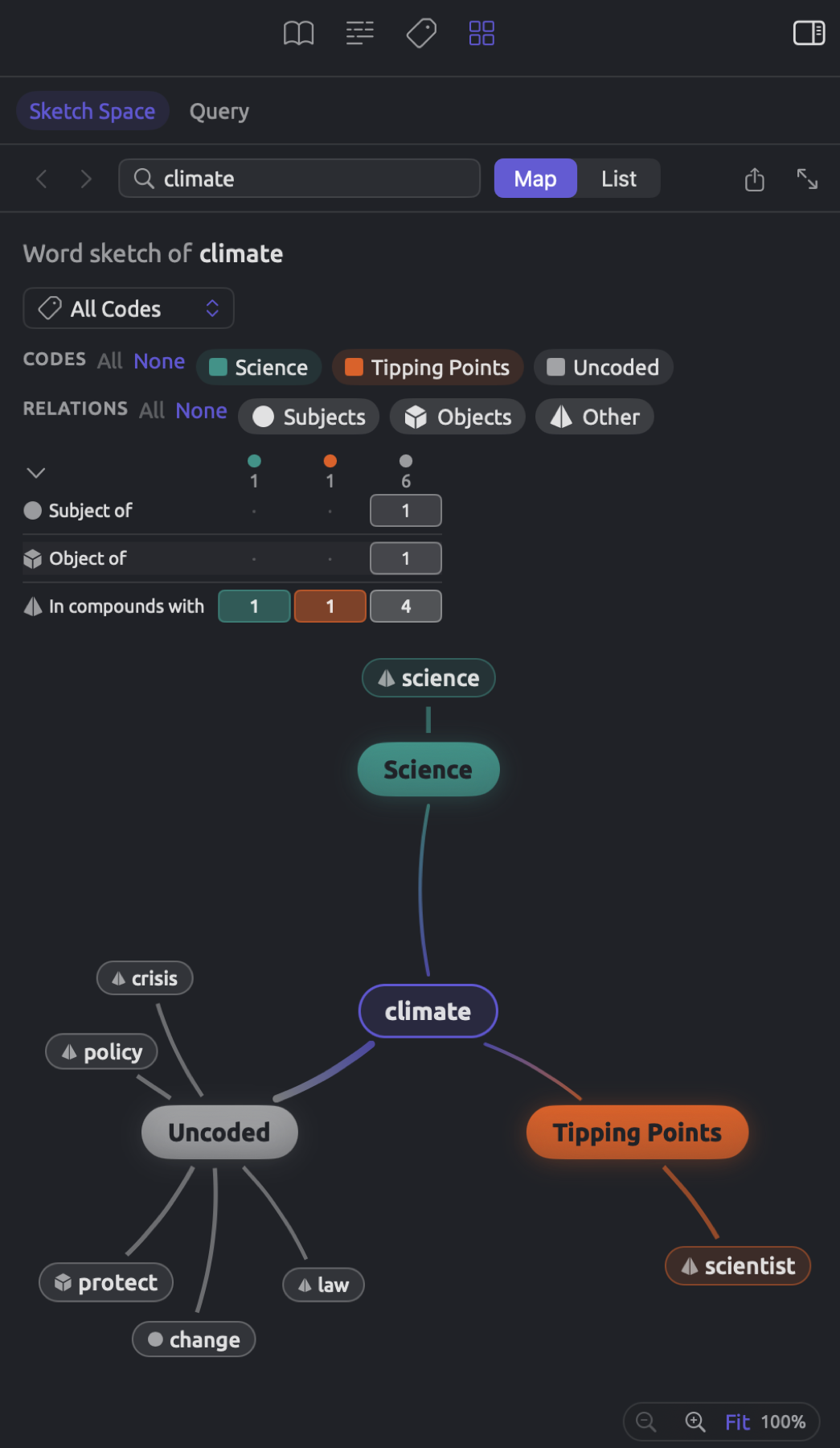
To investigate a word among all codes in a particular document:
- Open the document in the reader.
- Choose View ▸ Inspector ▸ Multimode (⌥⌘4). If Query is selected at the top of the tab, click Sketch Space beside it.
- Click a word in the reader. The line below the bar reads Word sketch of, followed by the word.
- Click a number in the grid or a word on the map to list its sentences.
Before choosing words in the reader, the tab says Sketch a Word. Should you pick multiple words, the tool will treat the main word of the phrase, the one the others depend on, as the center word; for instance, if picking the climate crisis, Sketch Space picks crisis as the center word. Each successive word that you pick thereafter becomes the new center word, while maintaining the choice of available codes.
The structure of Sketch Space includes, from top to bottom:
- The bar featuring the Back and Forward navigation controls, Word field, Map and List, export button, and Open in a window.
- The Word sketch of line containing the name of the center word and previously sketched words.
- Menu showing All Codes when the codes can be categorized differently.
- Codes legend containing one lenslet per column and the Relations legend consisting of one lenslet per sector.
- Relation grid.
- Comparison map or lists of partners in List display.
- Evidence list should you select any items.
This exact same bar is seen in the Word Sketch facet of the Grammar tab and the Code Sketch facet of the Coding tab. These three share the very same word and share a single history of navigation. Since the Web display belongs solely to the word sketch, the only options provided in Sketch Space are Map and List displays. Open in a window opens the document in the Word Sketch window, Multimode mode, with the word you chose earlier.
Should your document feature zero codings, Sketch Space informs you by means of No codings in this document yet. and displays a solitary Uncoded column (a normal word sketch). Should the word not participate in any grammatical relations whatsoever, you get a message saying No grammatical partners found for this word.
A memo linked to a passage and coded will itself constitute a coding, thus placing the passage within that code’s column.
Choosing the columns
Grouping the codes
Below the line Word sketch of is a menu for the codes that can become columns, which initially shows All Codes until something else is selected:
- All Codes includes all codes which apply to at least one instance of the center word.
- A parent code, e.g., “Urgency”, includes only its immediate subcodes, namely, “Tipping Points” and “Deadlines”.
- A code set, such as “Arguments”, includes all codes contained in the set.
The menu offers a parent code only if one of its subcodes includes the word. Similarly, it offers a code set only if it includes at least one code that does. Hence, for climate in “Running Out of Time”, the menu offers “Urgency” and “Arguments” apart from All Codes. This menu is shown if there is an option beyond All Codes; it will appear whenever there are attributes defined within a set or project (see Comparing attribute values). LemmaLoom saves each document’s choice.
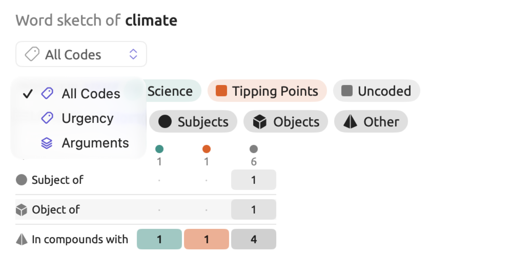
Selecting a parent code allows comparison between its subcodes, whereas selecting a code set allows comparison of codes from different parts of the code system.
A column counts only the codings of its own code, hence a subcode’s codings count in the subcode’s own column. For example, consider the passage in “Running Out of Time” that begins “Climate scientists speak of tipping points”. The passage is coded as “Tipping Points”, a subcode of “Urgency”. Hence, under All Codes in this example, the passage will appear in the column for “Tipping Points”.
Enabling and disabling columns
The Codes legend includes one lenslet per code covering the word in question, in the code’s color. Lenslets are ordered according to how often each code covers the word. The final lenslet is Uncoded, which appears in gray.
- Click on a lenslet to disable its column; click again to enable it.
- Selecting All will enable the first six columns. Selecting None will disable all columns. When there is no column enabled, Sketch Space displays No Partners.
- Shortcut menu (right-click) options include Enable only this, Disable (or Enable), and Enable all.
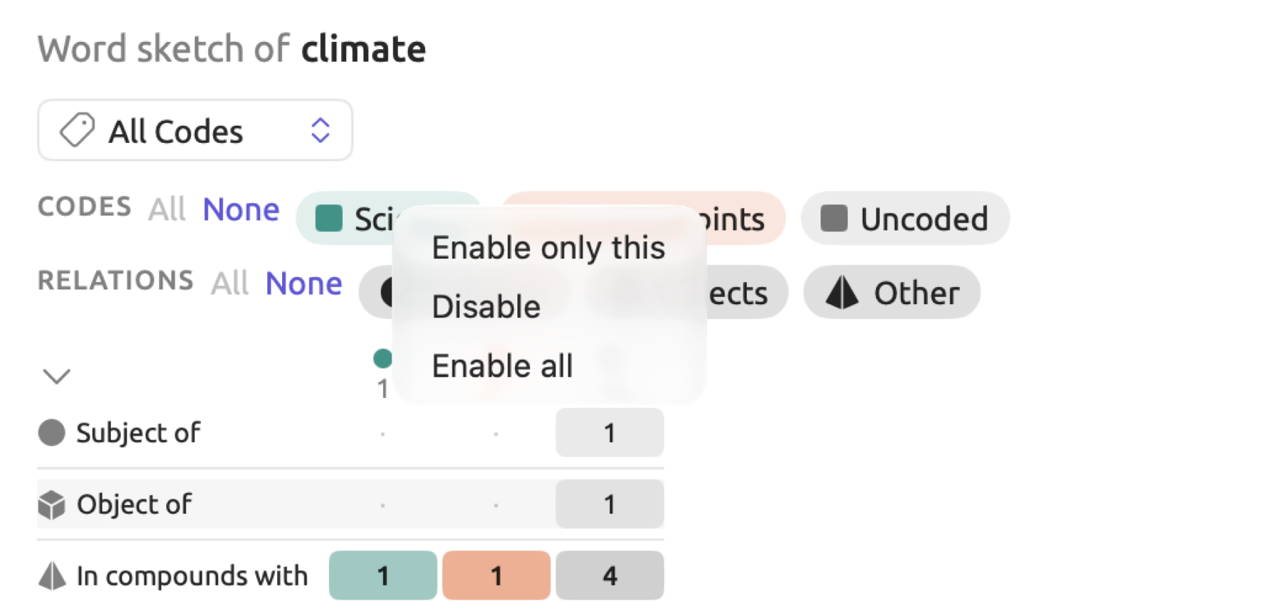
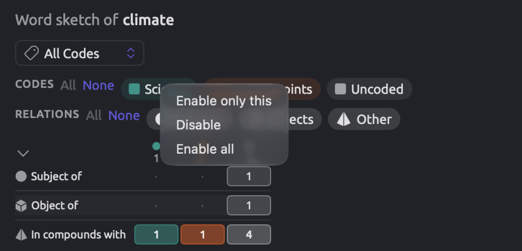
Sketch Space displays at most six columns at once. When there are already six columns displayed, enabling another will automatically disable the code column with the fewest occurrences of the word. The Uncoded column remains enabled. As a rule of thumb, it may be more visually comprehensible to observe two or three columns simultaneously rather than all six.
On your very first sketch of a word with All Codes, Sketch Space will display the top four codes covering that word, along with Uncoded. On selecting a parent code or a code set, Sketch Space displays a maximum of six codes within the selection, without including Uncoded. Occurrences covered only by codes outside the selection are then left out.
The relation grid
The grid displays data in a table form where there is one column for each code you show, and there is one row for each of the relations the word takes part in under those codes. It also shows how much of the column each relation accounts for.
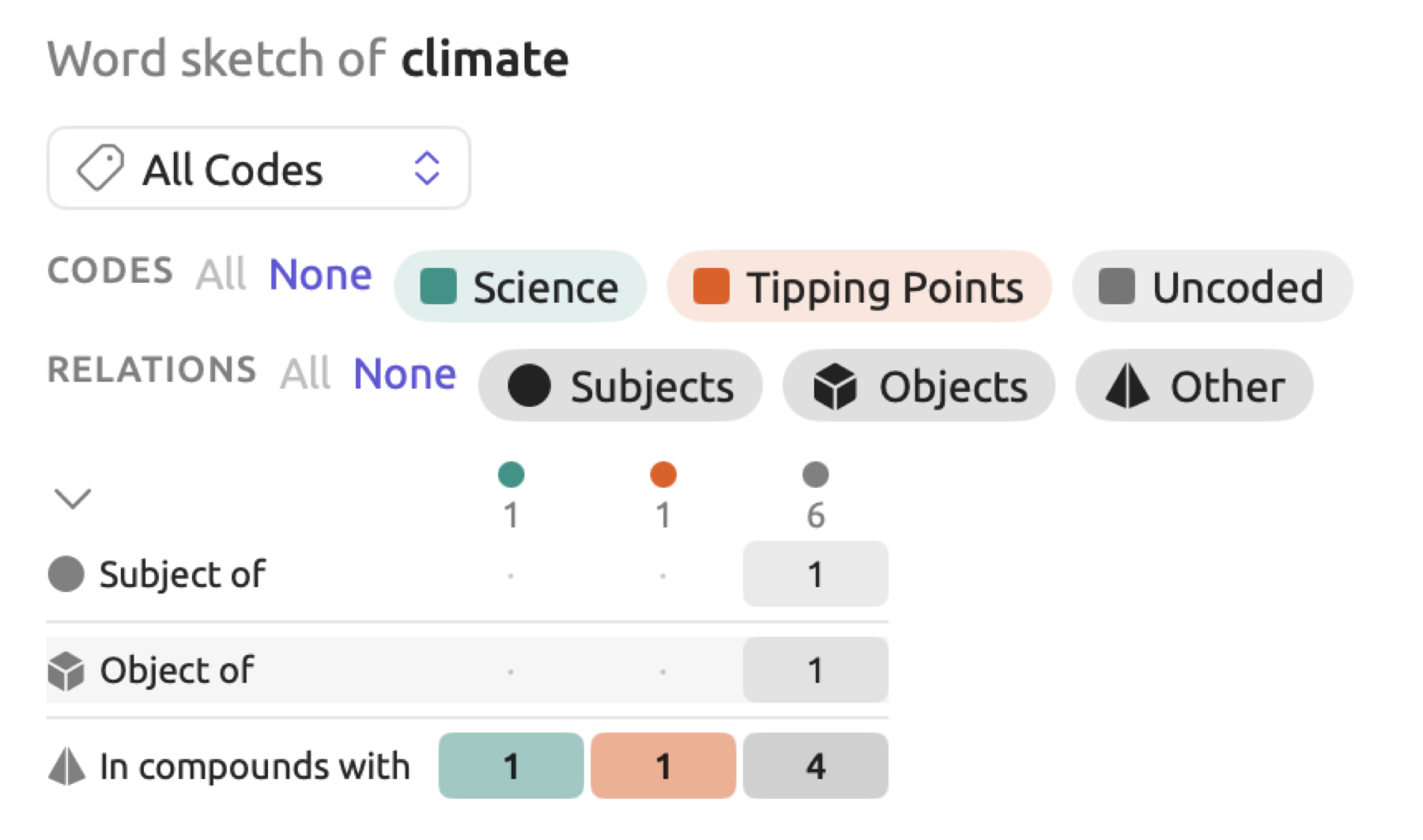
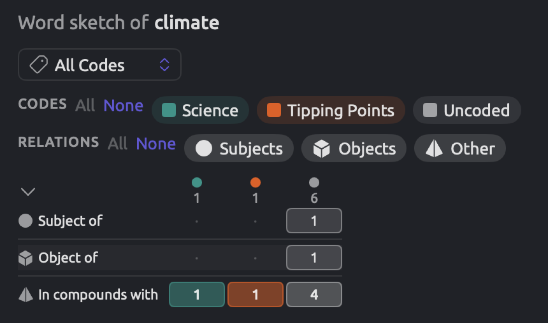
- The heading for each column tells you the color of the column along with the total count of occurrences of the center word within the column. The tooltip for a column heading will also show the name of the column, e.g., Uncoded · f=6, where f indicates the number of occurrences.
- In the rows, relations participated in by the word are presented consistently in order, each preceded by the symbol for their respective sectors. Lines delineate the boundary between sectors, with stripes marking every other row.
- Each cell presents the number of relations of its kind in the column, with · indicating zero counts.
- Shading of the cell reflects how much of the relations of the column are captured within it. A bold font indicates a ratio greater than or equal to 40 percent.
- The tooltip of a cell includes its count and the proportionate percentage within the column, e.g., In compounds with · Uncoded: f=4 · 67%.
While the number in a column heading counts occurrences of the word itself, cells are concerned solely with relations of those occurrences and thus may not agree with the count presented in their heading. In “a youth climate campaigner” of “Radio Debate”, the single occurrence of climate results in two relations in the In compounds with row due to being paired with both youth and campaigner. On the other hand, in “A Mayor’s Promise”, the occurrence found in “By 2035, this city will be climate neutral” contributes nothing, hence the “Deadlines” column there presents only dots. Lastly, in “Running Out of Time”, each occurrence provides exactly one relation.
Due to differences in sizes among columns, it makes more sense to evaluate shading and percentages rather than counts. All counts within a cell include relations regardless of whether the partner of such relations appears on the map or not.
An asterisk beside a count highlights a characteristic relation; a description follows beneath the grid (Characteristic relations).
Clicking a cell will retrieve the list of its sentences (covered later in The evidence list); hovering a mouse pointer above a relation name, a cell, or a column heading will highlight the matching partners on the map (see Brushing).
The collapsed grid
The chevron at the grid’s upper-left corner allows collapsing it into a profile with one row per column. Profiles compare columns while leaving more space for the map. Every row shows the column’s color, name, a bar, and the number of occurrences. The bar represents the distribution of relations across the five sectors. The segments range in shades of the column’s color according to their order from Subjects being darkest to Other being lightest. The length of each part of the bar reflects its percentage share of the total relation counts within the column. The bars are normalized based on the maximum occurrence number among the columns, meaning shorter bars imply smaller columns. A segment’s tooltip gives its sector and count.
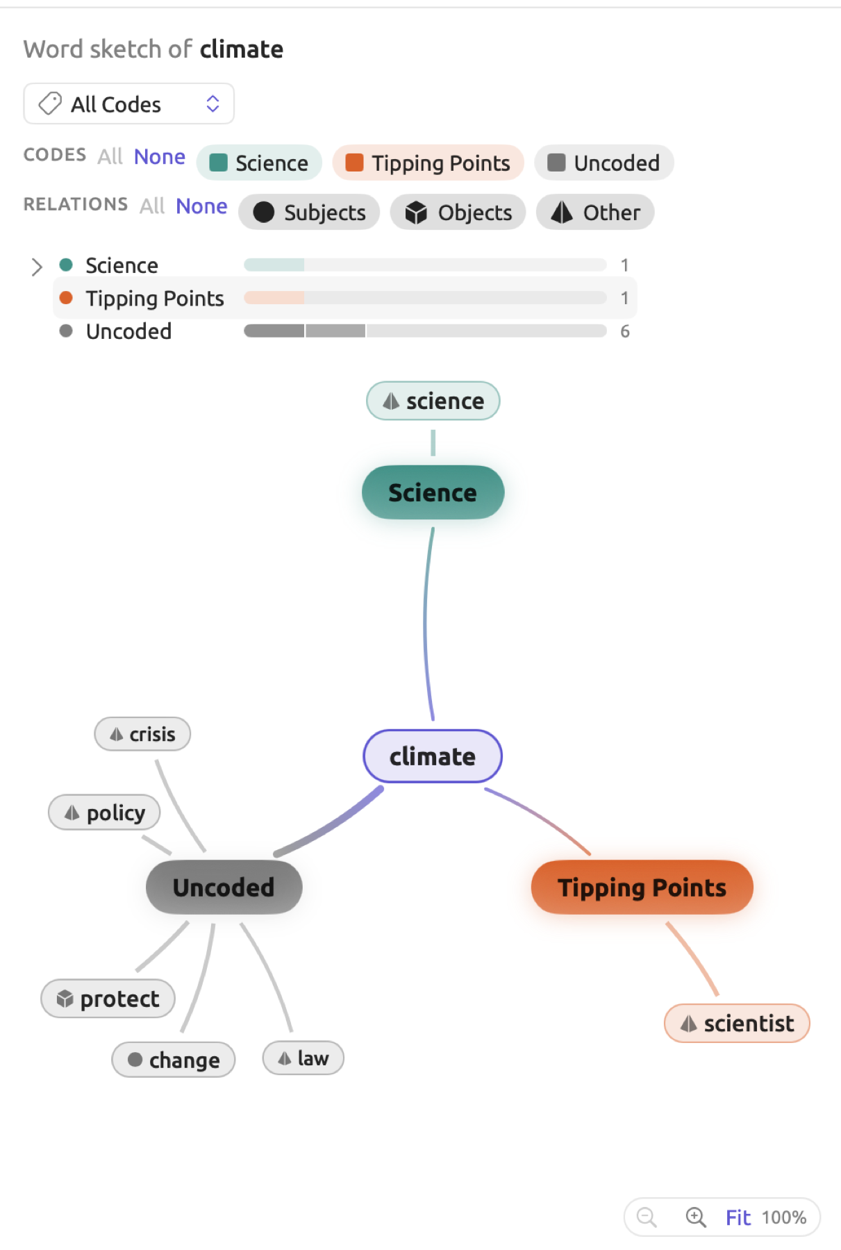
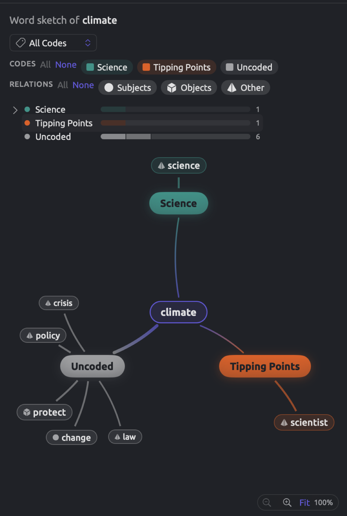
Clicking either a row or the chevron restores the grid’s expanded state. Within the Map display, the grid begins as collapsed should there be insufficient vertical screen real estate allocated toward the map area. Once you collapse or expand it yourself, your preference persists.
The comparison map
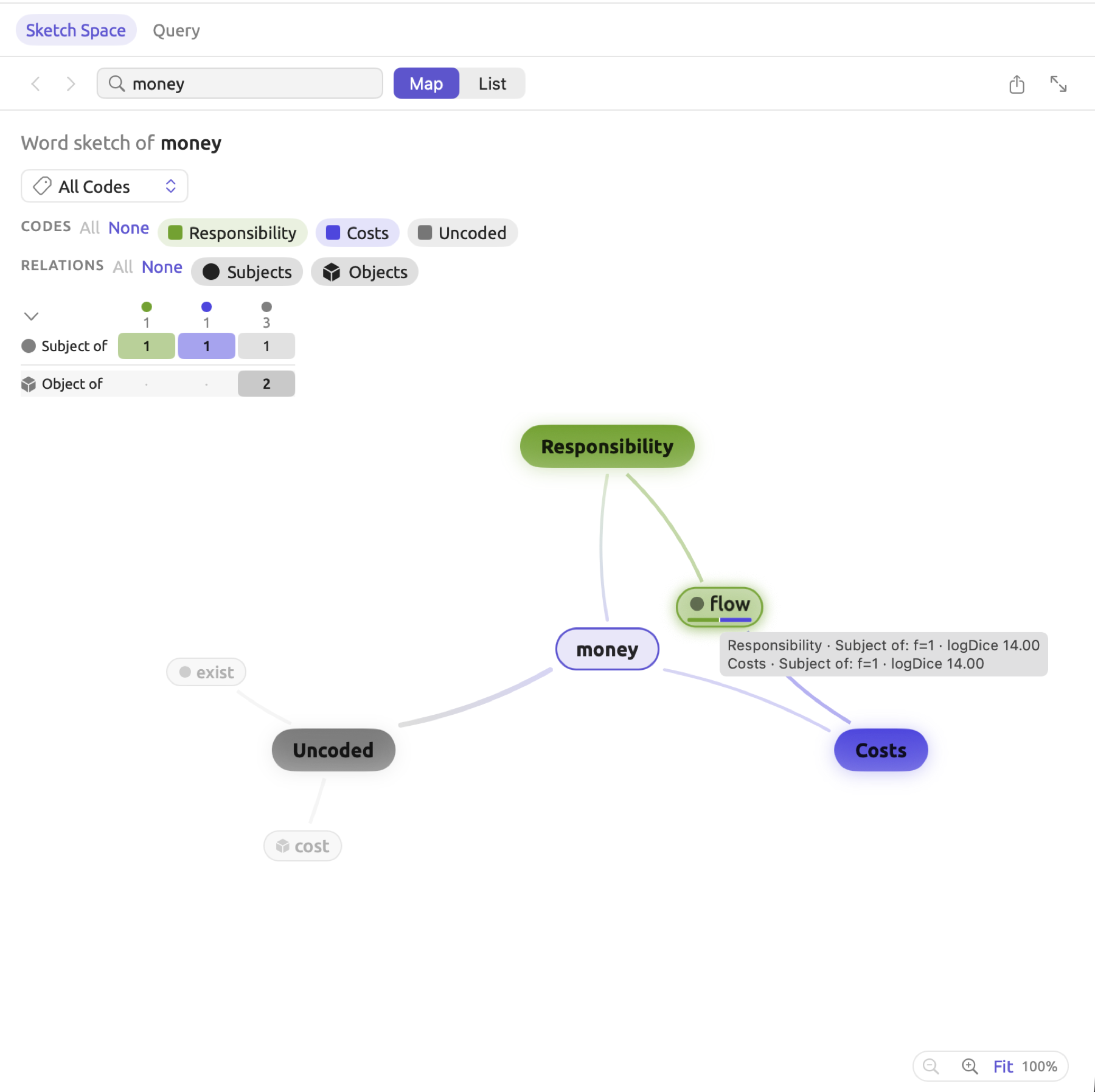
The map displays the hubs representing the columns you show, along with each hub’s strongest partners. Each hub is joined to the center word by a spoke, which is thicker when the column holds a larger share of the word’s occurrences. Each hub carries the column’s name and color; a long name is shortened with an ellipsis (…), and the hub’s tooltip gives the full name and the number of occurrences. A hub’s partners are ranked by the highest logDice each reaches in any relation, and up to 10 of them are shown, depending on the space available. A partner belonging exclusively to one hub sits on that hub’s outer side, away from the center. Partners that are among the strongest of several hubs sit between the hubs, with a line to each and a firmer outline. Underneath such a partner is displayed a colored bar indicating the proportion of co-occurrences of the partner with the center word within each column, while its tooltip reveals details of its associations in each hub, such as frequency and logDice. A larger typeface and heavier lines indicate a higher rank, while a symbol preceding each partner shows the sector(s) it belongs to.
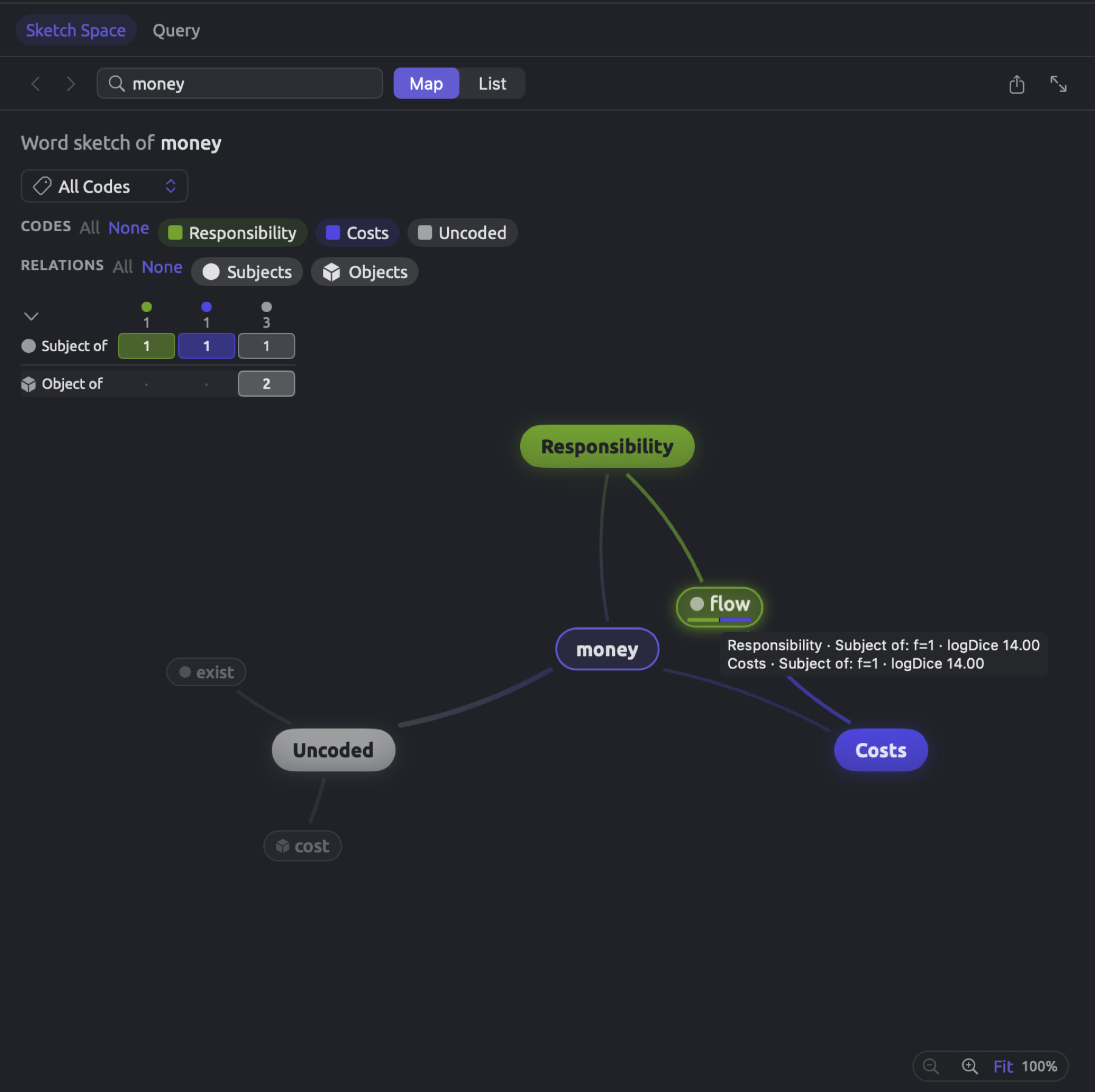
In the “Running Out of Time” example, each partner of climate connects to one particular hub, as each passage that includes the word carries at most one code; however, for money, its partner flow connects to both “Costs” and “Responsibility” due to the passage “then the money it raises should flow back to the households that pay it”, which carries both codes.
As you hover the mouse pointer over a partner, other partners fade. Its tooltip lists every association in a separate row per hub, with a relation label, frequency of the pair’s occurrences (f), and logDice.
As long as at least two columns keep partners in the sectors that are displayed, a hub whose column has none becomes disabled and its partners invisible.
Every relation within a column suggests its 12 strongest partners to the map. Within a single document, a partner only needs to appear alongside the center word once, whereas in a set or project it needs to occur at least twice in the same relation and column.
The map provides access to various functionalities:
- Clicking on a partner leads you to the list of all sentences featuring both the partner and center word in any of the shown columns (see The evidence list below).
- Shortcut menu options enable you to either change the center word with Sketch this word (see Sketching another word below), or navigate directly to the next occurrence of the partner in the reader with Show in context.
- Clicking on a hub allows you to focus on analyzing its corresponding column (see Drilling into a column below).
Zooming the map
The map will fit the available canvas space. If you want to examine the map in detail, there is a bar at its bottom right which contains the buttons Zoom out, Zoom in, and Fit, along with the current zoom level percentage. With a trackpad, pinch actions accomplish the same function, as does double tapping with two fingers to toggle back and forth between fitting and doubling the view size. Holding ⌘ while scrolling will also zoom in/out. After zooming in, dragging or scrolling moves the view. Changing the center word or the columns fits the map again.

A single column
In cases where only a single column contains partners, the map turns into a simple word sketch of the center word for that column. The center word is highlighted in the column’s color, and the partners of this word group themselves around it based on their relations to the center word. This is what you’ll see upon drilling into a column too.
Drilling into a column
Opening the drilldown of any particular column gives the word sketch of the center word within that column only, including all instances of it. Within “Running Out of Time”, clicking on the Uncoded hub for climate provides a word sketch of its six uncoded instances.
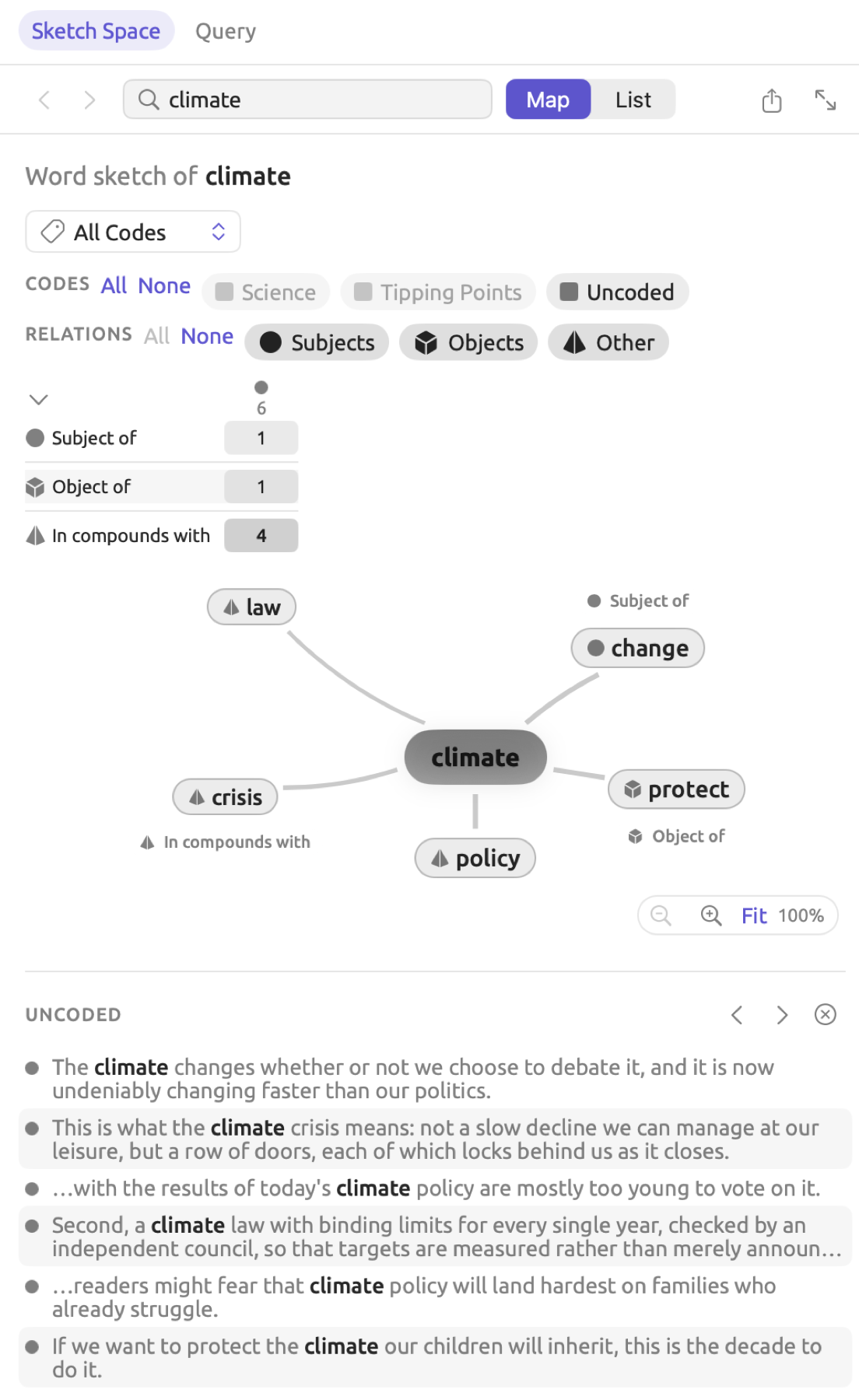
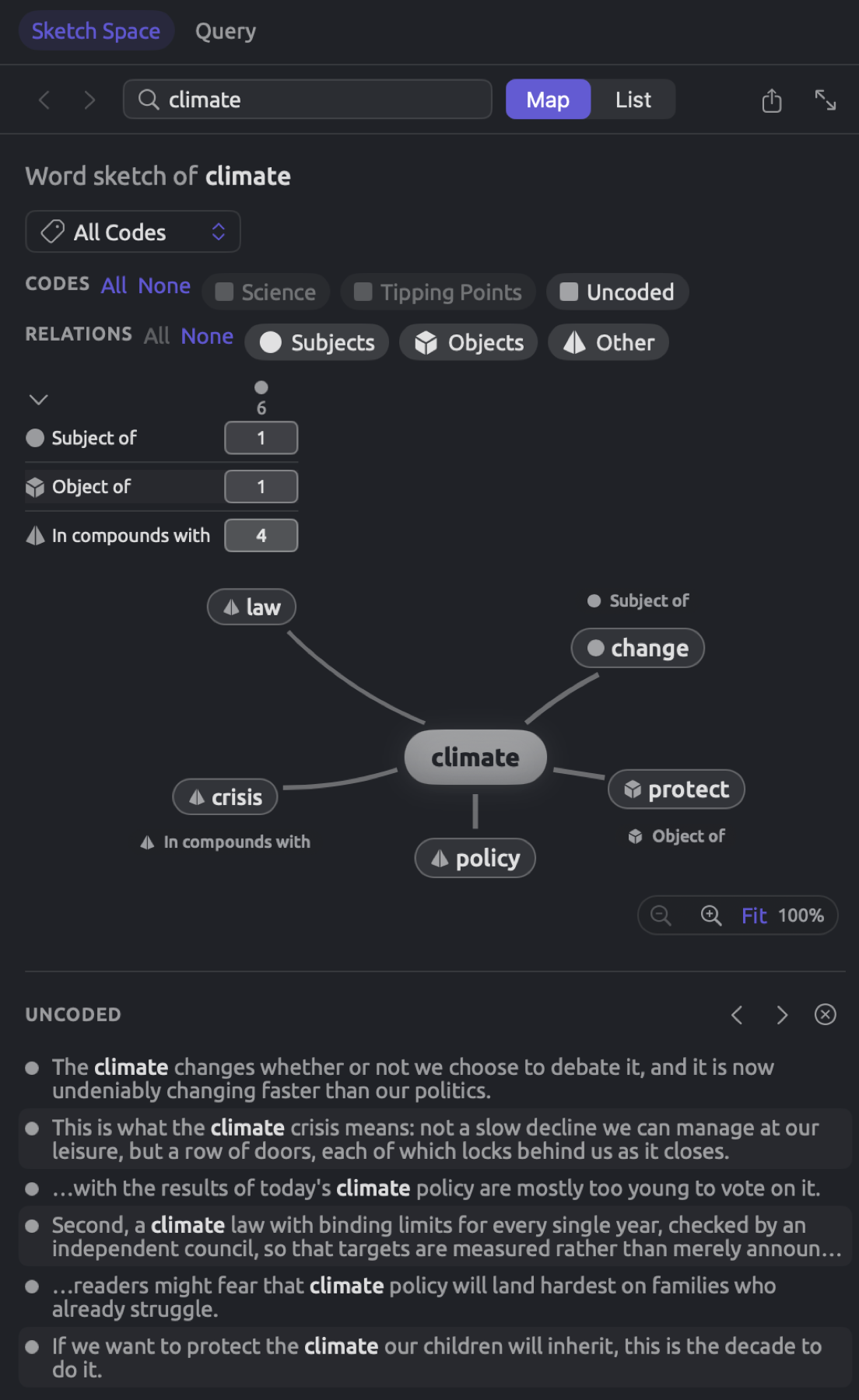
For the purpose of focusing solely on one column:
- Click its hub on the map. Sketch Space disables the other columns. The map shows the word sketch of the center word in that column, and the evidence list holds each of the column’s occurrences.
- To go back, click the center word, which now has the column’s color. The columns you had before return.
The way back ends once you toggle the columns or sectors differently. If you enable or disable a column or sector, or pick another item in the codes menu, clicking on the center word lists occurrences of the column instead. Reactivate the rest of the columns from the Codes legend.
The evidence list
The evidence list contains the sentences for what you have chosen. It opens below the map, or below the lists, when you select a grid cell, partner, or hub. The grid and the map remain above regardless. Resize the evidence list with the divider above it to increase or decrease its height.
| You select | Title | The list holds |
|---|---|---|
| A cell | the relation and column, such as In compounds with · Uncoded | every relation in the cell, including those whose partners are too weak for the map |
| A partner | the partner, such as policy | every occurrence of the pair in the columns and sectors you show |
| A hub | the column, such as Uncoded | every occurrence of the center word in the column; only the center word is bold |
Every row represents a single sentence. If the center word or partner sits far into the sentence, or the sentence is long, the row shows only the part around them, with an ellipsis (…) where text is cut. The center word and partner are shown in bold. On the left edge of each row are dots representing up to three codes, gray for uncoded occurrences. Rows are ordered according to reading order, and up to 100 rows are included in the list.
Selecting a row opens the corresponding sentence in the reader. The selected sentence is scrolled to, the center word is selected, and the pair is highlighted. Choosing a particular cell or partner takes the reader straight to the very first sentence of that choice.
The header contains:
- the ordinal of the sentence, like 2 of 4, once you’ve navigated to one;
- Previous match and Next match arrows, which step through the sentences and wrap around at the ends, past the first 100 if there are more; and
- Clear selection (a circled ×) for dismissing the list.
Selecting the chosen cell or partner once again works the same way as navigating via Next match.
Should any cell contain more than one partner, a line of buttons will be displayed right above the list with the strongest partners (max. 12, like on maps), along with the frequency count of each partner, such as policy 2. Selecting any of those buttons restricts sentence display to that particular partner alone, while selecting it again displays all partner sentences. If there are more than six, a last button such as +4 shows the rest.
Sectors
Relations between words belong to five sectors. Having divided relations into sectors allows you to study the linguistic behavior of the center word in a certain grammatical aspect, like whether it acts as a subject, for example, while ignoring other possible behaviors. In the Relations legend, you’ll notice the presence of lenslets belonging to every sector of relations the center word participates in. There is always a particular symbol associated with each sector, found in the grid, on the map, and in the lists. When there is no room for the names, the lenslets show only their symbols, and each lenslet’s tooltip gives its name.
| Sector | Symbol | Relations | Example for climate |
|---|---|---|---|
| Subjects | filled circle | Subjects, Subject of | the climate changes: Subject of change |
| Objects | cube | Objects, Object of, Complements, Complement of | protect the climate: Object of protect |
| Modifiers | triangle | Adjective modifiers, Adverb modifiers, Modifies | a changing climate: Adjective modifiers change |
| Prepositional phrases | rounded bar | Prepositional phrases | a climate without human-caused warming: Prepositional phrases without warming |
| Other | pyramid | In compounds with, Coordinated with | climate policy: In compounds with policy |
Object of lists the verbs which the center word acts as object for. Objects does the opposite; rather than listing the verbs acting on the center word, it lists the center word’s own objects. Hence, Objects populates itself whenever the center word is a verb like protect. Similarly, Subjects and Subject of, and Complements and Complement of, are paired in the same way. For more information on each relation, see Grammatical relations in Chapter 12, Word Sketch.
Disabling any sector by clicking its lenslet means that its partners will vanish from the map and the lists. Additionally, the sector’s rows fade in the grid, and a partner’s evidence list leaves out those relations. Exports leave out disabled sectors too. All and None enable and disable all sectors, respectively. Right-clicking a lenslet offers Enable only this. For example, to see only what the center word does as an object or complement in each column, right-click Objects and choose Enable only this.
Brushing
Grid brushing establishes a connection between your grid and map so that you can tell which partners belong to a particular row or cell in your grid without opening a list. When you hover your mouse pointer over sections of your grid, the corresponding partners remain highlighted on your map while the rest dim out:
- Over a relation name like In compounds with, all partners belonging to the relation in all shown columns.
- Over a grid cell, all partners associated with the cell.
- Over a column heading, all partners belonging to the column within all visible sectors of your map. In collapsed grids, rows of the profile do the same.
When your mouse pointer is hovering over In compounds with in “Running Out of Time”, science, scientist, crisis, policy, and law remain highlighted, but change and protect get dimmed. Once you have clicked a cell, the partners associated with the selected cell will stay highlighted while your mouse pointer is outside your grid.
Sketching another word
Changing the center word without leaving the comparison works as follows:
- Enter a word into the Word field and press Return. In the inspector, the field takes the word in whatever form you give it, so enter the dictionary form, e.g., scientist instead of scientists; the matching process ignores case, and another form yields the message No grammatical partners found for this word. In a set or project, it does not matter what form you enter.
- Right-click a partner on the map or in the list and click Sketch this word.
- In the inspector, pick another word from the reader.
Every word sketched is stored in a history, which displays in the line Word sketch of with the previous words separated by an arrow, e.g., climate › protect. You may click any previous word in order to revisit it or use the Back and Forward buttons in the bar; View ▸ Word Sketch ▸ Back (⌘[) and Forward (⌘]) do precisely that.
The List display
The List display replaces the Map display and uses lists to show your data. Clicking List in the bar will switch displays. The grid precedes the lists, which scroll along with the grid. Every visible column gets its own list, titled with its color, name, and number of occurrences.
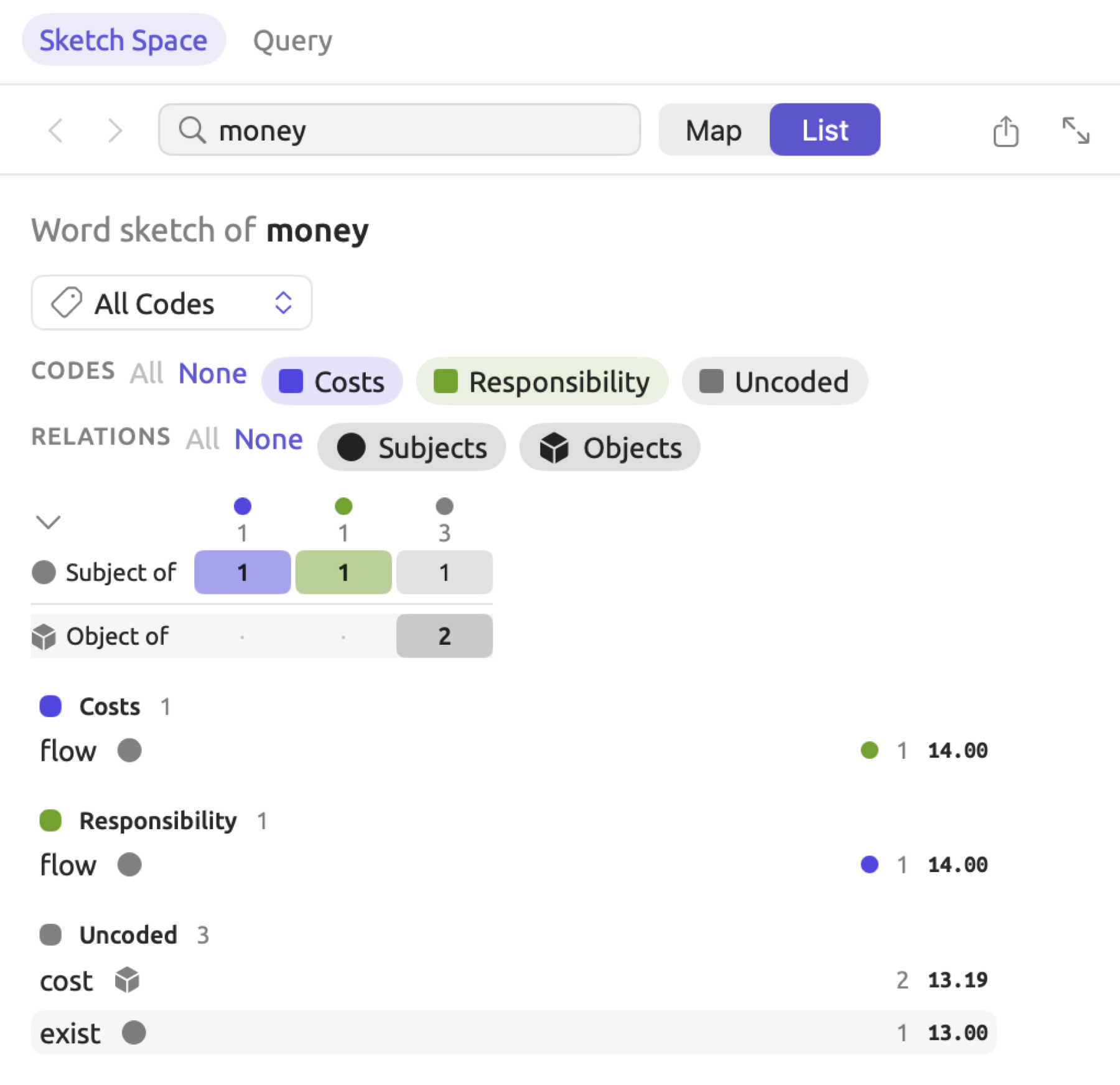
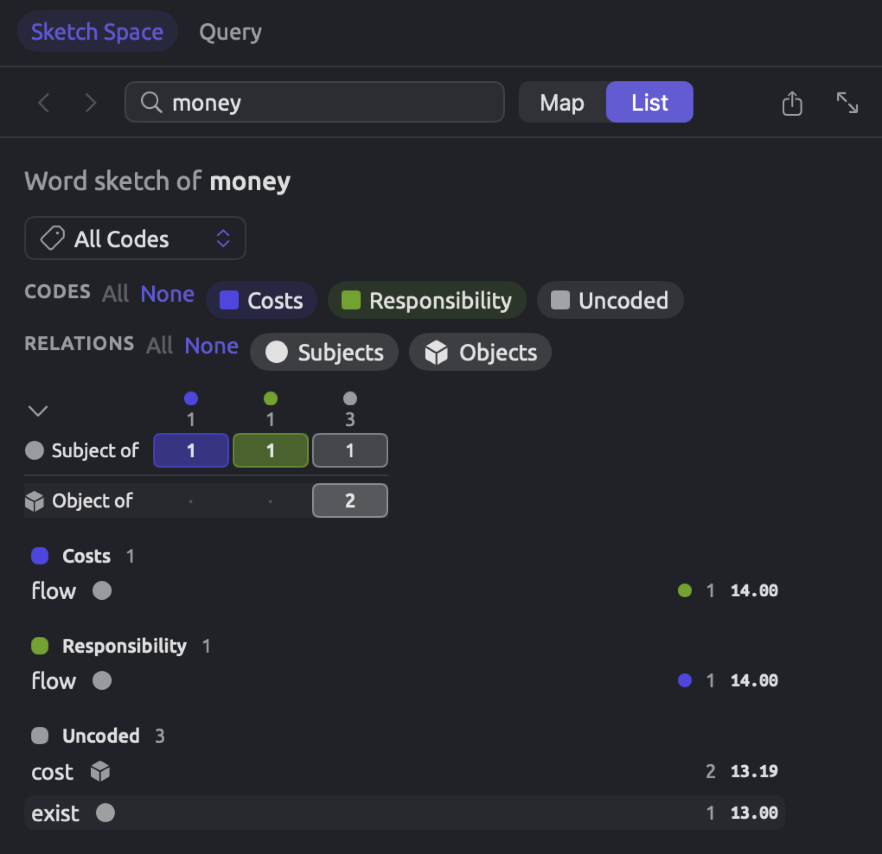
For each row, the list shows:
- The partner, followed by sector symbols.
- Colored circles for up to three other columns containing the same partner. A tooltip reveals their names.
- Occurrences of the partner appearing alongside the center word in this column, across all its relations.
- The logDice score achieved by the partner, the maximum among all its relations with the center word.
Rows are sorted based on score. Each section displays eight rows initially. Selecting Show all displays all available rows, while selecting Collapse hides all but the top eight rows. Hovering the mouse pointer over a row highlights the corresponding partner in all sections. Clicking on a row brings up its evidence list, and right-clicking it brings up the Sketch this word and Show in context commands.
When Sketch Space is very narrow, it always uses the List display. Map and List buttons are disabled, with tooltips saying Pane too narrow. Whether Map or List is selected will be passed on to the word sketch and the Code Sketch (see Chapter 12, Word Sketch). If Web is selected for the word sketch, Sketch Space uses Map.
Characteristic relations
There is a * marker next to a count if the occurrence frequency of the relation for that column exceeds the rest of the document significantly. In a set or project context, the comparison is done with the rest of the set or project instead. More information on statistical testing can be found in Chapter 12, Word Sketch.
The criteria for Sketch Space including a *, all of which must hold, are the following:
- There are at least three relations in a cell so that no * would appear on a cell with fewer.
- The relation in the column occurs more frequently than expected.
- The probability value returned from the one-sided Fisher’s exact test is lower than 0.05.
“Running Out of Time” does not have enough content for a *. Out of its cells for climate, only one has more than two relations, namely In compounds with under Uncoded. However, the column does not have higher frequencies of compound relations than the document as a whole, with 4 out of 6 versus 6 out of 8.
Consider instead another hypothetical longer op-ed piece in which climate takes part in 20 relations. Among all codes, there are only two covering this word (“Science” and “Costs”), and assuming no passage carries both, here are the numbers:
| Relation | Science | Costs | Uncoded | Whole document |
|---|---|---|---|---|
| Subject of | 3 | · | 2 | 5 |
| Object of | 2 | 1 | 1 | 4 |
| Adjective modifiers | 3 | · | · | 3 |
| Prepositional phrases | · | · | 2 | 2 |
| In compounds with | 1 | 4 * | 1 | 6 |
| All relations | 9 | 5 | 6 | 20 |
The final row and column contain totals, which were added here for illustrative purposes. Only the number 4 under In compounds with in the “Costs” column gets the * marker.
Expected counts
Across the entire document, climate takes part in 20 relations. Out of these, six (or 30%) of the relations are In compounds with. Assuming that the passages in “Costs” would use the term climate similarly to how it is used across the document, 30% of their five relations should be compounds. That equates to 1.5 relations; this figure is called the expected count. In “Costs”, there are actually 4 relations of In compounds with.
The formula to calculate the expected count is as follows:
Where:
- = expected count of the current cell
- = total number of relations of this column (five in “Costs”)
- = total number of relations of this row in the whole document (six for In compounds with)
- = number of relations of the center word in the whole document (twenty)
gives the share of the particular relation in all relations in the document. For “Costs”, .
The one-sided Fisher’s exact test
That there are four relations but an expectation of 1.5 sounds like quite a difference. “Costs”, however, only contains five relations, and with so few numbers, random variations affect the counts a good deal. Fisher’s exact test determines how likely it is for randomness alone to obtain this high a count.
The test considers each cell as a table of four counts:
| In compounds with | Other relations | Total | |
|---|---|---|---|
| Costs | 4 | 1 | 5 |
| Rest of the document | 2 | 13 | 15 |
| Total | 6 | 14 | 20 |
Consider the 20 relations as 20 playing cards where 6 cards are labeled In compounds with (compound cards). Shuffle the deck of 20 cards and draw 5 random cards into a hand designated “Costs”. In the absence of connection between coding and grammar, the relations in “Costs” would be such a random hand. The hypothesis test seeks the probability of getting 4 or more compound cards in “Costs”.
When calculating the number of ways in which cards can be chosen from without taking the order into consideration, the combinations formula gives
read “n choose r”, where is the factorial function, denoted by the sign following the number. The factorial refers to the multiplication of integers beginning from one up to the number itself. Thus, . For instance, two out of four cards can be picked in different ways, namely AB, AC, AD, BC, BD, and CD.
Choosing five cards out of twenty, , will involve many terms above and below the fraction line that will cancel. Only the first five terms above the line and the five below it remain,
Thus, there are 15,504 different possible combinations of five-card hands from 20 distinct cards. A hand with exactly four compound cards involves picking 4 cards out of six in ways, multiplied by choosing the fifth, non-compound card from the remaining fourteen cards. , and thus . A hand of exactly five compound cards involves picking five cards out of six, , and zero cards from the fourteen others (); hence 6 total. Consequently, 216 hands satisfy the criteria, and the p-value is
Counting for all the possible numbers of compound cards shows how unusual the value 4 is:
| Compound cards in the hand | Hands | Share of all hands |
|---|---|---|
| 0 | 2,002 | 0.129 |
| 1 | 6,006 | 0.387 |
| 2 | 5,460 | 0.352 |
| 3 | 1,820 | 0.117 |
| 4 | 210 | 0.014 |
| 5 | 6 | 0.0004 |
Most random hands hold one or two compound cards, as the expected count of 1.5 suggests. Random hands containing four or more compound cards occur in only around 14 hands per 1,000.
The ratio here is referred to as the p-value, the probability of observing a value greater than or equal to the value in question if the column were drawn randomly from the word’s relations. The p-value is not the likelihood of an effect existing, however. When is below 0.05 (that is, a count would arise fewer than five times in 100 draws), Sketch Space adds a *, indicating significant deviation. The threshold value of 0.05 is merely a tradition practiced commonly in the social sciences. With a p-value of 0.014, “Costs” has obtained a * on its In compounds with count.
The formula for calculating the p-value involves summing the fraction for every count starting from the observed value.
Where:
- is the count of the observed cell. The value for “Costs” is 4.
- is each integer from (inclusive) up to the limit , indicated underneath and above , respectively. The sign means “add up the fraction for each of these values of ”.
- is the number of ways of choosing items among possibilities. This corresponds to choosing which compounds will be used.
- counts the ways of choosing the remaining entries in the column among . These would be non-compounds.
- counts all possibilities of drawing items out of . This corresponds to all the possible combinations.
- is the minimum between and , meaning no hand has more than items or more compounds than the that exist.
As such, the of “Costs” ranges from 4 to 5 (5 being the smaller of 6 and 5). Their corresponding fractions are and , respectively.
The test is one-sided in nature since it searches for values only above what is expected. A relation that occurs in a column less frequently than anticipated will never get a *. Additionally, the test is exact as it considers every possible hand.
Two counts without an asterisk
“Science” has three relations under Subject of, out of nine overall. Given five Subject of relations in total, the expectation is . While three is greater than this expectation, it is close. If nine cards were dealt from twenty, five being Subject of, then for taking on values between three and five inclusive, the probability of being greater than or equal to three would be:
In random circumstances, “Science” should get three or more Subject of relations approximately 40 times in 100. No * marks appear here, since the probability of a random hand having three or more is high.
All three Adjective modifiers relations in the document belong to “Science”. The expected count is . Now takes only the value three, as there are only three such relations, and the probability would be:
There is no *, since the probability of getting all three Adjective modifiers is 0.074, above 0.05, or about 7 times in 100. Yet no other column has Adjective modifiers relations.
Reading the asterisk
A * indicates that the count would be unusually high if the column represented a random sample of the word’s relations. The reason behind it is not explained, however.
Tests are conducted individually for each cell. In a grid containing six columns and twelve relations, the maximum number of cells is 72. Even in those cases where no real difference exists, up to 1 out of every 20 cells can receive a *. A large grid may therefore display a stray * or two.
For testing, the relations are treated like individual cards shuffled randomly in a deck. Documents are different from that, however; writers tend to repeat themselves, and a single paragraph coded “Costs” could provide multiple relations involving the exact same partner. Repeating oneself increases the chances of receiving a * beyond what the p-value indicates.
An absence of * does not necessarily indicate similarity among the columns either. With smaller columns, the test usually fails to reach 0.05; refer to the Adjective modifiers example above for illustration. When the test is done with larger sets or projects, which can involve thousands of relations, even small differences receive * markers. Note, however, that the * symbol does not describe how big the difference is. Instead, you should compare the cells’ percentages yourself.
Your own codes create the columns, which means that any occurrences coded “Costs” partly because they referred to a climate levy or a climate tax include an intrinsic connection to In compounds with. When an occurrence relates to two different codes, the occurrence gets counted twice, once in each corresponding column. Hence, the two columns are not independent groups.
Refer to Chapter 13, Analyzing Codes and Chapter 16, Query Results and Statistics for guidance on comparing document groups via statistics.
Sketch Space for sets and projects
For your set, tag, or even whole project, Sketch Space analyzes every document simultaneously. With several documents, the number of occurrences in your columns becomes large enough for differences to stand out.
Opening Sketch Space for a set or project
Open the Word Sketch view for the material you want to compare, in one of these ways:
- For the project, click Word Sketch under Project in the navigation sidebar.
- In the sidebar, click the set or tag, then click Word Sketch among the buttons in its tab.
- Right-click on either the project, a set, or a tag in the sidebar, and click Word Sketch. This opens the Word Sketch window.
- Type a word in the Word field and press Return. Any form will do, so scientists finds scientist.
- Click Multimode in the mode control, next to Grammar and Coding, or choose View ▸ Word Sketch ▸ Multimode (⌘3). For more information on the other two modes, see Chapter 12, Word Sketch.
While preparing documents, LemmaLoom displays Preparing, along with a count of prepared documents.
All three modes share the bar at the top, which contains the Back and Forward buttons, the Word field, the mode control, the Map, List, and Web options, and the export button. The Web option is disabled in Multimode, and upon hovering, its tooltip reads Web is not available in this mode. Opening the Word Sketch view in the Word Sketch window requires clicking the Open in a window button, located at the rightmost edge of the bar, with two arrows going diagonally across it.
When documents in your scope contain translations, you will find a menu next to the export button, showing Originals initially, with the tooltip Source. Under Corpus, this menu allows you to toggle the corpus used for analysis among Originals, as well as each translation language; for instance, you may find Translations (German). See Chapter 12, Word Sketch for additional information on translation corpora. Within the Word Sketch window, the menu appears regardless of whether there are translations or not. Within this menu, the Scope section switches between the project level, set or tag level, and the document open in the reader. The menu then shows the scope’s name, such as “Climate Debate”, followed by the corpus when translations are included. Once the document is selected, Sketch Space behaves similarly to its counterpart in the inspector, except that you change the center word with the Word field or Sketch this word.
Everything explained above for a single document applies here as well, but with slight modifications:
- Unindexed documents are omitted during analysis. At the bottom, LemmaLoom notes how many documents are included, for example 13 of 14 documents indexed.
- Changing the center word involves typing in the Word field or using Sketch this word.
- The center word applies to all three modes and persists after switching between modes.
- To qualify for appearing on the map or lists, the partner needs to occur at least twice in the same relation and column. Single occurrences still count in the grid, though.
- In evidence lists, titles precede each document’s sentences. Clicking a row opens the document in the reader and shows the particular sentence.
- A * compares the column with the rest of the set or project.
- If there are no codings in any document in the scope, the note reads No Codings.
Document codes
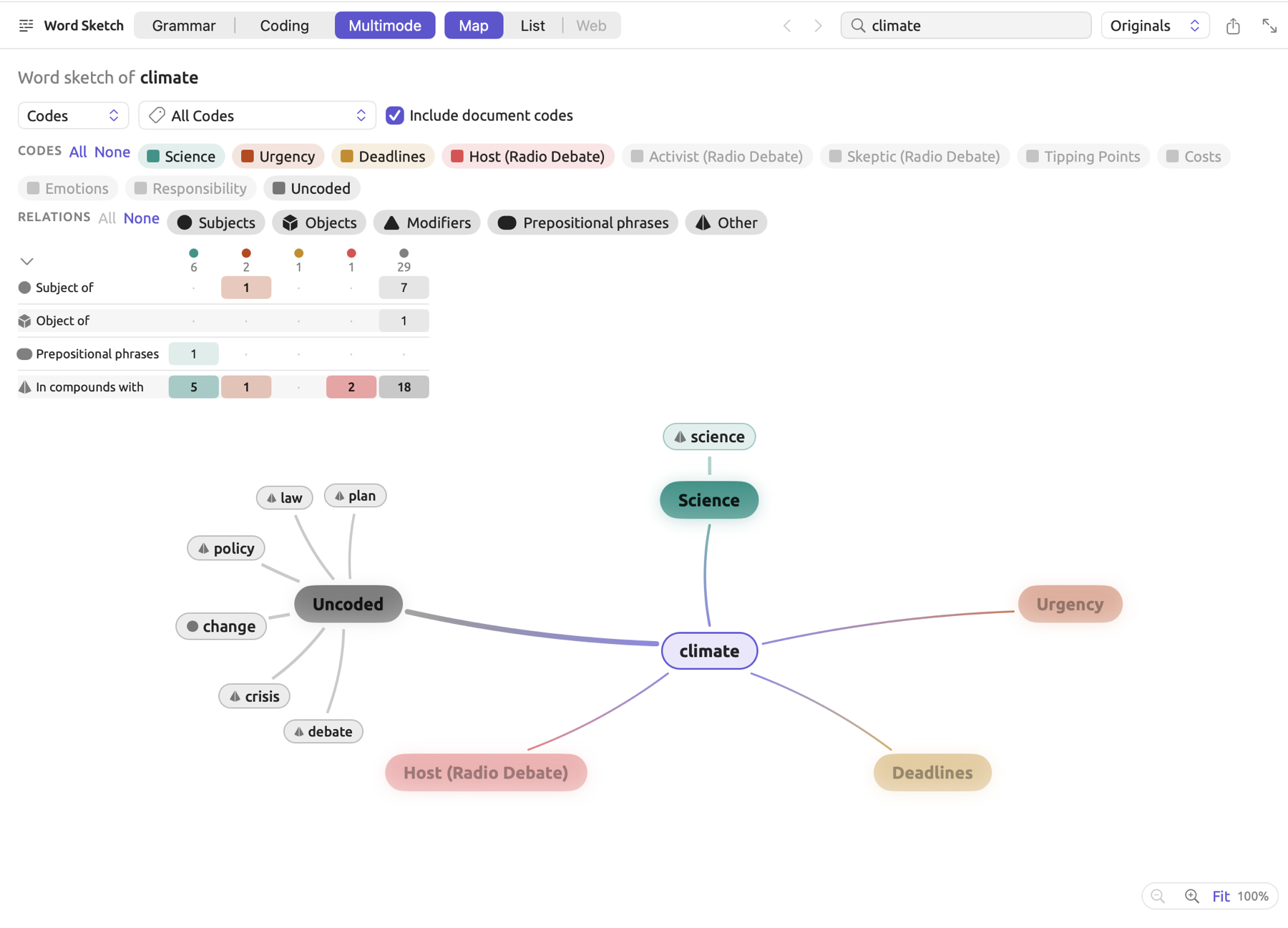
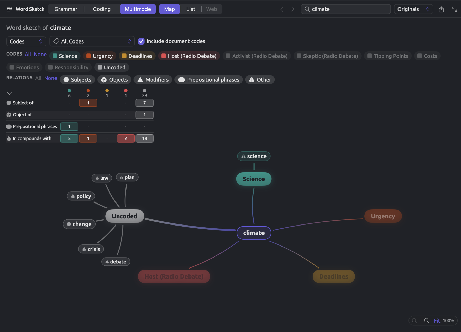
A code can be confined to a particular document, too, as seen in Chapter 7, Coding. If there are such codes in any documents contained within a set or a project, the latter shows their names with the document’s title in parentheses afterward, shortened when the title is long, to indicate this restriction. As seen in the “Climate Debate” project, for instance, there are codes specifically for each speaker of “Radio Debate”. Hence, the project’s columns can include “Host (Radio Debate)”.
If documents within the scope of your analysis have codes of their own, the Include document codes checkbox appears right beside the codes menu. It comes pre-selected with a tooltip saying Also group partners by codes that belong to a single document. You should keep this checkbox selected whenever these codes contribute toward answering your question, like those of the speakers in “Radio Debate”, and deselect it otherwise. When deselected, occurrences coded this way would still contribute toward any code other than these on the passage, or toward Uncoded. This checkbox and the one in the Coding mode are the same setting.
Comparing attribute values
Attribute columns in a set or project consist of document attribute values as opposed to codes, and each column stores occurrences of the center word in documents that fall under that particular attribute value, coded or not. They should be used whenever your question concerns attributes of the document itself, such as who wrote it or where it appeared.
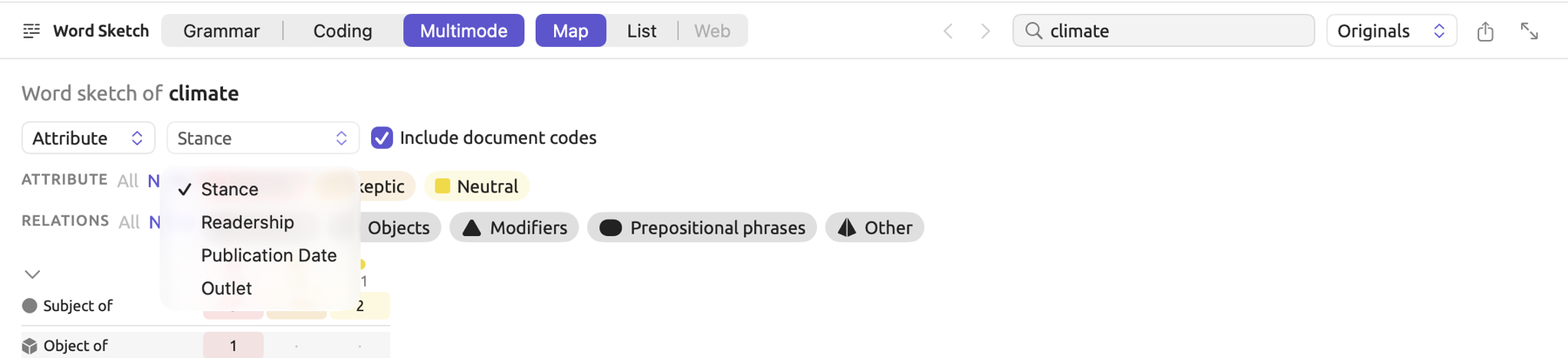
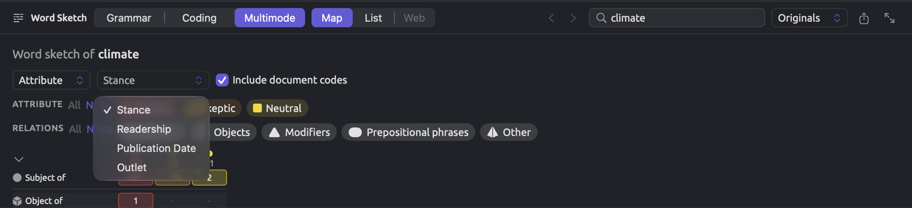
The “Climate Debate” project contains several attributes including “Stance” (“Activist”, “Skeptic”, or “Neutral”), “Readership”, and “Outlet”, among others. The following figure compares climate mentions among all three “Stance” values.
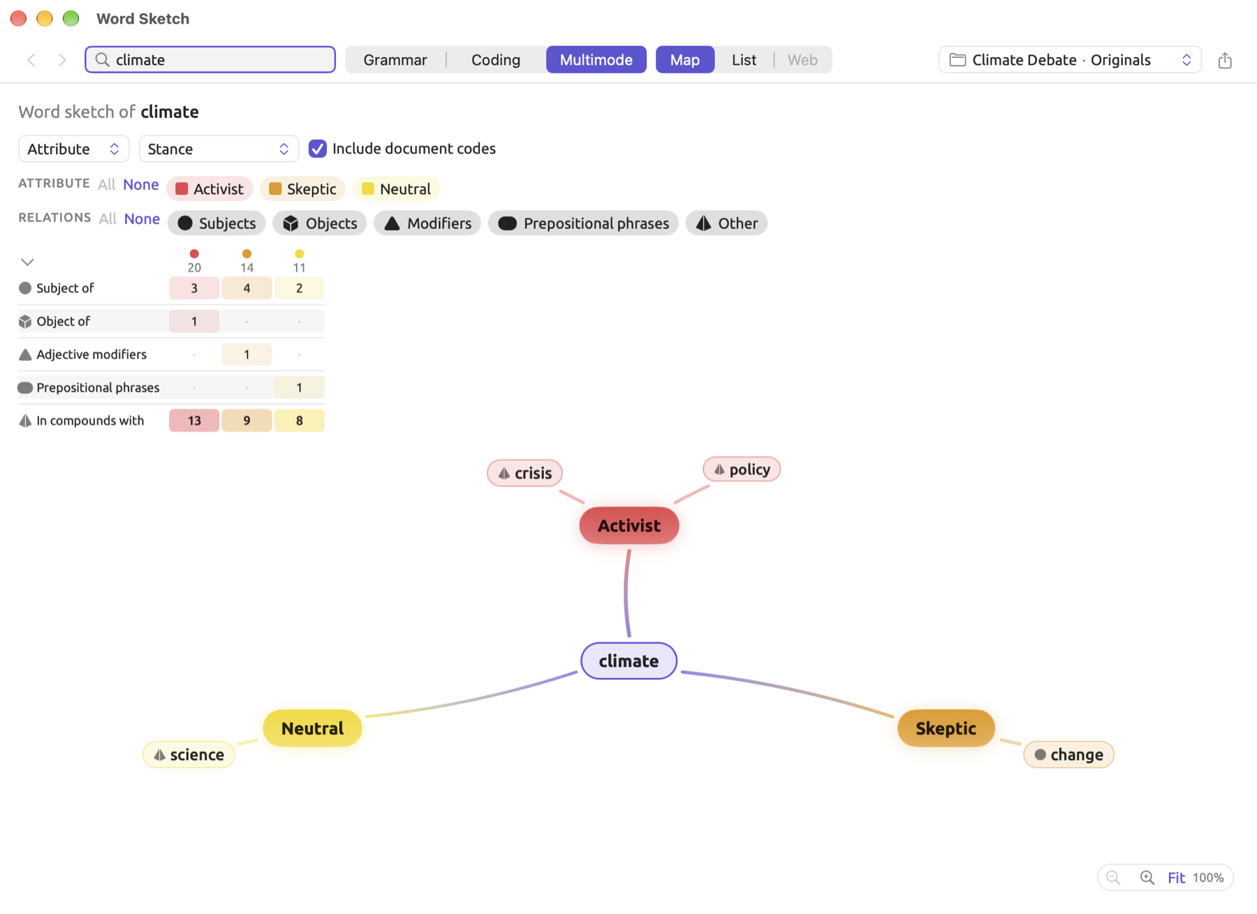
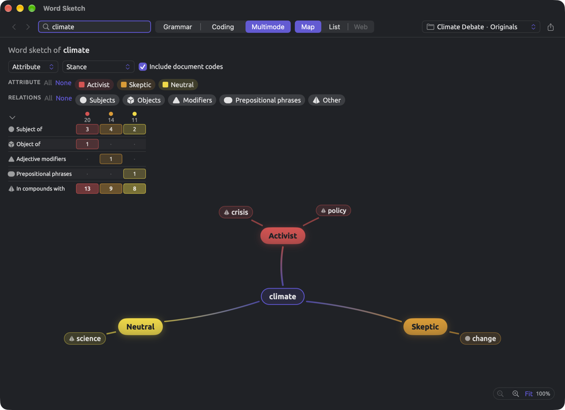
For comparing a word based on the values of an attribute:
- Open Sketch Space for a set or the project, and sketch the word.
- Below the line Word sketch of, click the menu that shows Codes, to the left of All Codes, and choose Attribute. This menu appears when the project has attributes. A second menu appears beside it, showing the name of the first attribute.
- In the second menu, choose the attribute whose values you want as columns.
The legend, now renamed Attribute, contains one lenslet for every value. Documents without a value will form the final column named No value.
How the values turn into columns depends on the attribute’s type:
| Type | Columns |
|---|---|
| Text | one per value |
| Picker | one per value, in the order of the picker’s options |
| Boolean | Yes and No |
| Integer and Decimal | up to four ranges, each holding about a quarter of the documents |
| Date | one per year |
When working with numbers, LemmaLoom ranks the value of each document within the scope, and it places three range boundaries. It multiplies the number of values by ¼, ½, and ¾, discards the fractional part, and chooses the value after that many. Within the “Climate Debate” project, the fourteen original documents have “Readership” values of 3.1k, 8.5k, 23k, 41k, 57k, 68k, 72k, 96k, 186k, 254k, 310k, 398k, 412k, and 875k. For the highest boundary, 14 × ¾ = 10.5; hence, it becomes the 11th value. The boundaries become the 4th, 8th, and 11th values, namely 41,000, 96,000, and 310,000. The columns are, therefore, < 41000, 41000 to under 96000, 96000 to under 310000, and ≥ 310000, containing 3, 4, 3, and 4 documents, respectively.
Repetition of values might cause two boundaries to converge into one, leaving fewer ranges. Where most of the documents possess the lowest value, so no boundary exceeds this value, Sketch Space creates columns for individual values instead.
A translation contributes with the value of its original document. Column colors are taken in order from the code color palette, and evidence list dots display these colors accordingly.
Like code columns, attribute columns possess similar characteristics. At most six columns appear on screen at a time, and the first six values that occur are displayed initially. A * indicates that documents under the column use the relation more often than other documents in the scope. Note, however, that it may rest upon the occurrences within only one document because it is counted by relation rather than document; thus, it is necessary to look into the document headings within the evidence list. Selecting Codes or Attribute in the first menu, or changing the attribute, closes the evidence list immediately.
Select any attribute whose values differ within the scope. Each document under the “Activists” set possesses “Stance” value “Activist”; hence, comparison should be done based on “Readership” or “Outlet”.
Exporting
In the bar at the top of Sketch Space, there is a button of a square icon with an upward arrow; it saves what Sketch Space shows. While there is nothing to export, the button becomes disabled, and its tooltip becomes Nothing to export.
- In the Map display mode, clicking this button shows a menu. PNG and PDF save a picture of the map itself; CSV saves the data table.
- In the List display mode, clicking the button will prompt a save dialog for the CSV table directly.


Whatever visualizations you have in the Map display, including the current columns and sector settings, will be included in the exported picture.
For a CSV export, the exported table will consist of rows corresponding to each partner in each relation and column, and the headers will be Code (or Attribute), Relation, Collocate, Lemma, Part of speech, Frequency, and logDice. Collocate is the partner as shown in the visualization, such as without warming; Lemma is its dictionary form. Only each cell’s top 12 partners available for maps will be exported, and disabled columns and sectors are left out.
As usual, a save dialog asks you to provide a location to store the exported file. Its default filename suggestion will be based on sketch-space- and the center word, sketch-space-climate for instance.