Statistics at a Glance
This appendix compiles the metrics shown throughout LemmaLoom, such as the readability metrics in the Text tab in the inspector, and the p-value resulting from comparing the texts produced by the activists and the skeptics. Each table uses terminology presented by the software, with references back to chapters where each metric has been covered with examples.
Short definitions of many of these metrics can also be found in Help ▸ Glossary, in the categories Text statistics and Association measures.
Where the numbers appear
| Place | Numbers | Explained in |
|---|---|---|
| Text tab, Overview | Counts, readability, vocabulary, syntax, and structure of one document | Chapter 10, The Text Inspector |
| Grammar tab, Collocates | Four association scores; the CSV export adds three more and the expected count | Chapter 11, The Grammar Inspector |
| Grammar tab, Word Sketch; Coding tab, Code Sketch; the Word Sketch view and window | f (frequency) and logDice for each partner | Chapter 12, Word Sketch |
| Multimode tab, Sketch Space; the Multimode mode of the Word Sketch | Counts and shares of relations, the *, and logDice in the list | Chapter 14, Sketch Space |
| Coding tab, Code Stats | Segments and coverage of each code; φ and * for overlapping codes | Chapter 13, Analyzing Codes |
| Codebook and Code Stats in the shelf | Segments, Documents, Coverage | Chapter 7, Coding; Chapter 13, Analyzing Codes |
| Code Matrix in the shelf | Counts; with Group columns by, counts or percentages and a test for each code | Chapter 13, Analyzing Codes |
| Relations in the shelf | φ and * for each pair of codes, and the number of overlaps | Chapter 13, Analyzing Codes |
| Count, Compare, and Over Time in queries | Measures, Range, DP, and tests | Chapter 16, Query Results and Statistics |
| Collocates and Keywords in queries | Seven association scores; log-likelihood and log ratio | Chapter 16, Query Results and Statistics |
| Queries sorted by Score | The score of each passage | Chapter 17, Query Patterns and Discovery |
| Network in queries | Counts of linked hits for each pair of values | Chapter 16, Query Results and Statistics |
| Form × Function, Discourse, Category Frequencies in the Dictionaries section, Attribute Breakdowns in Code Stats | Plain counts | Chapter 11, The Grammar Inspector; Chapter 19, Dictionaries; Chapter 13, Analyzing Codes |
A short primer
Examples throughout this primer will refer to the project entitled “Climate Debate”, included as the example project. In particular, the Code Matrix example refers to actual codings from the example project; these can be seen by importing the example project via File ▸ Import ▸ Example Project. The rest of the numbers are invented but consistent, chosen to keep the arithmetic simple.
Counts, shares, and rates
A count is a measurement representing the occurrences of something. For instance, you could measure 20 occurrences of hedges in “Radio Debate”, or 6 codings of “Urgency” within the “Activists” set. All measurements in LemmaLoom stem directly or indirectly from a count.
Share, on the other hand, is the proportion between parts and the whole they are contained within. Shares run between 0 and 1 and are most commonly expressed as percentages. Share measures in LemmaLoom include coverage, Lexical density, the Share measure for queries, and the percentages used in a Code Matrix. Suppose “Costs” codings span 250 characters out of the 5,000 characters of “Running Out of Time”. Thus, the coverage share for “Costs” equals , which means 5.0%.
Rates are similar to shares in that they are ratios, yet their divisor is text length. Rates require scaling for readability:
Here, represents the count while stands for the number of words. Dividing yields hits per word, a very small number. Multiplied by 10,000, rates become hits per 10,000 words, the exact scale used by the Per 10,000 Words measure in queries.
Take for example “Radio Debate” with 800 words and 20 hedges, and “Let’s Not Panic” with 600 words and 18 hedges. This gives:
Whereas the first uses more hedges, the second uses fewer hedges but at a higher rate. Particle density calculates rates per 100 words, just like several of the equations used in readability scores. On a scale of 100 words, both rates become 2.5 and 3.0, respectively. It follows, then, that the ranking does not change.
If you need to calculate the rate of occurrence for a whole group of documents, you can calculate either the pooled or document-specific rates. Pooled rates take the total number of occurrences divided by the total word counts. Long documents therefore carry greater weight than shorter ones. The rows of a query show these rates. The alternative method calculates individual rates and ranks them against each other. The rank test in Compare uses this method (see Tests later in this chapter).
Logarithms
The logarithm is an expression of the power to which a number called the base must be raised to get another number. LemmaLoom uses three bases:
- Log base 10 of 1,000 is 3 () because .
- Log base 2 (also abbreviated ) represents the number of doublings involved; hence, as .
- Natural log, abbreviated , has , the number that starts with 2.718, as its base, and is the ln button on your calculator.
Regardless of the choice of base, the logarithm of 1 always evaluates to 0. A value above 1 gives you a positive logarithm, while one smaller than 1 yields a negative logarithm, provided it is larger than 0. Zeros cannot give you a logarithm, nor can negative numbers. For this reason, some formulas add 0.5 to the count or omit all zeros.
In comparing ratios with each other, logarithms can prove useful. “Four times as often” and “a quarter as often” lie equally distant from “as often”, but on a linear scale, the distance between 4 and 1 amounts to 3 points, while that between 1 and 0.25 lies short of a point. Logarithms of base-2 will yield 2 and −2 respectively, lying equidistant from 0:
| Ratio | 1/8 | 1/4 | 1/2 | 1 | 2 | 4 | 8 |
|---|---|---|---|---|---|---|---|
| −3 | −2 | −1 | 0 | 1 | 2 | 3 |
Base 2 logs () are used for the log ratio scale, MI, and logDice scales because one unit corresponds to either twice as much or half as much. For the Log-Likelihood scale, is used. Interpretation of the log-likelihood statistic in relation to a cutoff level can be done via chi-square values associated with p-value thresholds (see p-values below).
For those calculators without capabilities, divide the value by after pressing the ln button (). So, for instance, since while , then , indicating just above one doubling.
Expected counts
Many statistics involve comparing what you have discovered with what you would discover had nothing separated the groups. This latter value is known as the expected count.
If the activist texts total 4,000 words while the skeptic texts contain 3,000 words, and the word hope occurs 12 times in the former but 2 times in the latter, the values take on the form shown below in tabular format:
| hope | Other words | Words | |
|---|---|---|---|
| Activists | 12 | 3,988 | 4,000 |
| Skeptics | 2 | 2,998 | 3,000 |
| Total | 14 | 6,986 | 7,000 |
When both groups use the word hope at the same rate, its 14 instances should be distributed in proportion to word counts. Since the activists’ documents contain four-sevenths of all the words, they are expected to have 14 × 4/7 = 8 instances of hope; the skeptics, 6 instances. The expected count of a cell can generally be found by multiplying its row and column totals together, then dividing by the grand total:
In the case of the activists’ hope, . Thus, while the activists have 12 uses, which is 4 more than expected, the skeptics only have 2 uses, which is 4 less than expected. The expected count is simply an average, hence it may not always yield integers.
The chi-square statistic χ² sums the squared differences between each cell’s count and its expected count , each divided by :
Here, is a cell’s observed count, is the cell’s expected count, and the symbol means “add up over all the cells”. Squaring makes differences in either direction contribute positively to the result. Dividing by the expected count allows differences to contribute more to the final score in small cells than in large ones. The expected counts for the other words amount to 3,992 and 2,994, which both differ from actual counts by 4. As such,
Keywords, collocates, chi-square tests, the * in Sketch Space, and φ of overlapping codes begin from calculating the expected counts. However, they vary according to what constitutes a row or column. Keyword lists have rows representing two document groups. Collocates’ rows correspond to words inside and outside the windows. Overlapping codes’ rows pertain to characters inside and outside each code.
p-values
In general, there will almost always be some discrepancy between two groups’ usage rates of a particular word, regardless of whether there is anything to distinguish one group from another. This discrepancy can be assessed statistically in order to test its significance, and p-values range from 0 to 1 to express the probability of a difference at least this large if the groups did not really differ. If your p-value is low, then the discrepancy is hard to put down to randomness alone.
Log-likelihood for a keyword list in LemmaLoom’s queries (see How the two scores are calculated in Chapter 16, Query Results and Statistics) is twice the sum of the products of each observed frequency and the natural logarithm of its ratio to the expected frequency. In notation form, this is written , as shown below for hope.
Note that measures roughly the same departure from expectations that the chi-square statistic does, with differences in methodology and values being fairly minimal; compare 5.34 to the earlier 4.68.
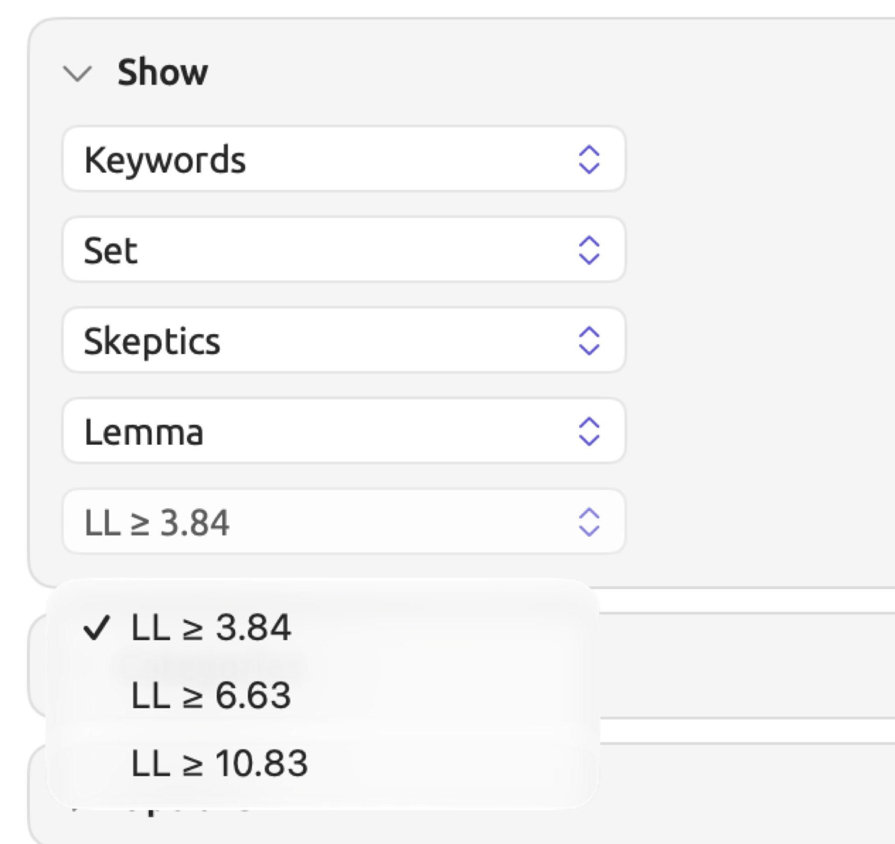
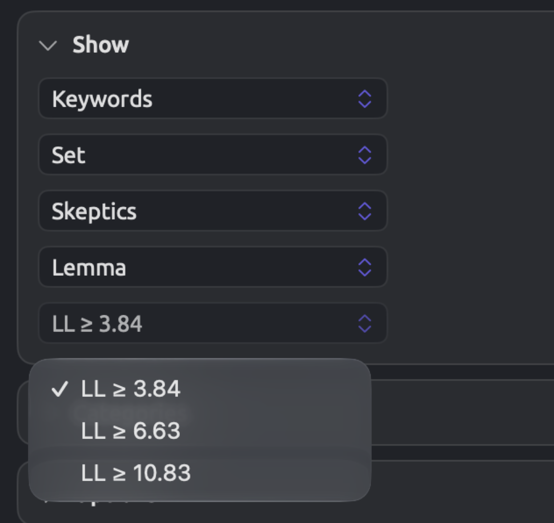
At the observed of 5.34, there is roughly a 0.021 probability that a difference of this size or larger occurs simply by chance, when both groups use hope at the same rate. Out of every 100 instances where the difference between both groups’ usage rate was zero, you might expect about two instances like this one, so hope passes the threshold LL ≥ 3.84 but not LL ≥ 6.63.
P-values of 0.05, 0.01, and 0.001 are typically chosen for significance; any p-value below 0.05 is often considered statistically significant. The threshold p-value of 0.05 is used by LemmaLoom wherever it shows significance (see How significance is shown later in this chapter).
A p-value of 0.021 is not equivalent to a 98% probability that there is indeed a difference. A p-value does not indicate the magnitude of the effect; rather, the effect size is used for this purpose (see Effect sizes below). Neither does a p-value greater than 0.05 show equivalence between the two groups; with a limited number of documents, a sizable difference could slip past without reaching statistical significance.
A p-value also makes an assumption that there was only one test conducted. A keyword list runs one for every word. For example, if 1,000 words that show no real difference undergo a hypothesis test, about 50 (5 in 100) will appear to be statistically significant at LL ≥ 3.84 purely by coincidence. More conservative criteria like LL ≥ 6.63 only admit roughly 10 words in the same circumstances, whereas LL ≥ 10.83 admits about 1.
Most hypothesis tests require comparing the calculated value against a distribution. The distribution provides the likelihood, for every value of the test statistic, of obtaining that particular outcome when the groups do not differ; the p-value corresponds to the portion of the distribution beyond that point. Normal distributions are used for the rank test for two groups. Chi-square distributions are used for the rank test for more groups, chi-square tests, and keyword thresholds.
Unlike other tests, Fisher’s exact test calculates the actual p-value of the test statistic rather than estimating it approximately. All arrangements of cells that retain the marginal sums are accounted for, adding their probabilities together for outcomes no more likely than the observation. As such, it remains a valid approach for cases where chi-square distributions are known to fit poorly, specifically those where the expected counts are relatively low (under five or so, by a common rule of thumb).
A two-sided test considers deviations from expectations in both directions, whereas a one-sided test accounts for one direction alone. Compare in queries and the Code Matrix employ two-sided Fisher’s exact tests. Conversely, the Sketch Space feature uses one-sided tests, which look only for more relations than expected, as does the Multimode mode of the Word Sketch.
The specific shape of a chi-square distribution depends upon its degrees of freedom (df). Tables containing rows and columns have degrees of freedom equal to ; fixing the row and column sums leaves only that many cells free to change. Rank tests with groups require . Here are some of the minimum values for meeting each cutoff:
| df | p = 0.05 | p = 0.01 | p = 0.001 |
|---|---|---|---|
| 1 | 3.84 | 6.63 | 10.83 |
| 2 | 5.99 | 9.21 | 13.82 |
| 3 | 7.81 | 11.34 | 16.27 |
| 4 | 9.49 | 13.28 | 18.47 |
The first row stores the three values in the menu showing LL ≥ 3.84 in keyword lists. These three values are also the usual threshold values for interpreting the log-likelihood of a collocate.
Effect sizes
A p-value is a combination of both the magnitude of your difference and the amount of evidence you have for it. Effect sizes measure only the magnitude of your difference, independent of the number of documents.
Take the Code Matrix of “Climate Debate” with its columns grouped by Group, which gives two groups, “Print” and “Online”. The first switch, which chooses what each cell counts, is set to Documents (see Grouping the columns in Chapter 13, Analyzing Codes). Six documents are in “Print” and six in “Online”. “Heat Wave Report 2024” and “Carbon Tax Debate” form the column Ungrouped, which the test leaves out. Two of the print documents (“Running Out of Time” and “Net Zero Will Cost You”) and all six online documents have a “Deadlines” coding:
| With “Deadlines” | Without | Documents | |
|---|---|---|---|
| 2 | 4 | 6 | |
| Online | 6 | 0 | 6 |
| Total | 8 | 4 | 12 |
The table will yield expected counts of in the first cell and 2, 4, and 2 in the other cells, respectively. Every observed count differs by 2 from its expected count, and , yielding a χ² of
This χ² statistic exceeds the critical value for the 0.05 significance level of 3.84. However, since there are only two groups, the Code Matrix will employ Fisher’s exact test instead, which handles very small expected cell counts. The resulting probability value will be . The effect size is , wherein is your sample of 12 documents. φ is listed in the Cramér’s V column.
Consider now that your study is repeated on ten times as many cases as before while preserving the same proportion of your counts. Thus you observe 20 out of 60 print documents and 60 out of 60 online documents. As a consequence, your chi-square statistic becomes ten times greater than before at 60.0, with p below 0.001. However, φ remains equal to 0.71 since proportions were unchanged.
| Effect size | Reported with | Formula | Values | Rough reading |
|---|---|---|---|---|
| r | The rank test for two groups | 0 to below 1 (see Small groups below) | 0.1 small, 0.3 medium, 0.5 large | |
| ε² | The rank test for three or more groups | 0 to 1 | On a squared scale, 0.01 small, 0.09 medium, 0.25 large | |
| φ | Fisher’s exact test in Compare; overlapping codes in the Code Stats facet and in Relations | 0 to 1 | 0.1 small, 0.3 medium, 0.5 large | |
| Cramér’s V | Chi-square tests in Compare, where the test line shows it as V; the Code Matrix | 0 to 1 | As φ for tables with two columns; in larger tables, smaller values already count as large | |
| Log ratio | Keywords | See Keyword and profile scores below | No limit; 0 means no difference | 1 is twice as often, −1 half as often |
represents the total number of observations counted by each test. Documents are observed in the rank tests, the presence test, and the Code Matrix. Words are observed in Chi-Square on Counts, and for a table under Compare, the hits in its cells. Characters are observed in overlapping codes when testing for significance of overlaps between codes. and χ² stand for the statistic values of the tests. stands for the minimum of either the number of rows or the number of columns. measures how far U lies from the value chance would give, , in standard deviations, the typical distance of U from that value:
and represent the document counts of the two groups respectively, while equals without the sign.
Ranks
Some tests are ranking-based. That means each value receives a rank based upon its ordering. Four documents whose rates are 22, 30, 30, and 41 would have ranks of 1, 2.5, 2.5, and 4. Ranks of 2 and 3 would be taken up by both 30s; thus, they share the average of .
Note how ranks disregard spacing between values. If the maximum rate changes from 41 to 410, its rank remains unchanged at 4. That is why one document with an extreme rate cannot determine the outcome of the rank test on its own.
Document statistics
The Overview facet of the inspector’s Text tab (⌥⌘1) provides access to the statistics of the active document once it has been indexed. All statistics are listed according to five sections titled Overview, Readability, Lexical, Syntax, and Structure. Bar graphs of Parts of speech, Functions, and Phrases come afterward. The statistics of Type-token ratio, MATTR, and Mean dependency distance are all displayed with two decimal places, while LIX is displayed as a whole number. Hapax ratio and the shares are whole percentages, while the remaining statistics are shown with one decimal place. Queries provide access to these statistics through the document field Statistic, and thus allow filtering or grouping based on statistical properties (see Finding documents by a statistic in Chapter 10, The Text Inspector).
Here, words means word tokens; this measure does not account for punctuation symbols or other non-word characters like #, but includes numbers. Sentences refer to sentences identified during indexing by LemmaLoom.
Counts and structure
| Statistic | What it measures | Values |
|---|---|---|
| Sentences | The sentences in the document | Whole number |
| Words | The word tokens | Whole number |
| Unique words | The different words, counted by lemma (dictionary form), so cost and costs count once | Whole number, at most Words |
| Paragraphs | The paragraphs, divided at blank lines when the text has any, and otherwise at every line break | Whole number |
| Characters | The characters of the text, spaces and line breaks included | Whole number |
| Avg. sentence length | Words divided by sentences | Words, with one decimal |
| Dialogue share | The share of words inside quotation marks, estimated by pairing them | 0% to 100% |
| Questions and exclamations | The share of sentences that end in a question mark or an exclamation mark | 0% to 100% |
| Sentences per paragraph | Sentences divided by paragraphs | 1 or more in practice |
| Parts of speech, Functions, Phrases | Words by word class and by grammatical function; phrases by kind | Whole numbers |
The first five stats fall under Overview. Avg. sentence length introduces the Readability section, followed by the next three stats under Structure. Counts and Structure in Chapter 10, The Text Inspector explain how each statistic works in detail.
When analyzing transcripts, sentence boundaries are defined according to transcription, which means that any statistic based on sentences is influenced by the transcriber’s choice of punctuation.
Readability
A readability formula estimates the difficulty level of the text based on average sentence lengths and word lengths. Which readability formulas appear varies according to which language is used for the document.
All the readability formulas follow notation used in Chapter 10, The Text Inspector. represents the number of words while is the number of sentences. Syllable counts are , letter counts , and letters/digits counts . Three-or-more syllable words are counted for and three-or-more syllable words without proper nouns for . Longer-than-six-letter words are counted for while one-syllable words are counted for .
| Statistic | Language | Formula | Reading |
|---|---|---|---|
| Flesch Reading Ease | English | Higher is easier. Flesch’s own scale runs from very difficult (0–30) to very easy (90–100); the app’s note puts plain English at 60–70. Values can fall outside 0–100 | |
| Flesch-Kincaid Grade | English | A US school grade (grade 8 is about age 13 to 14) | |
| Gunning Fog | English | Years of schooling | |
| SMOG | English | A US school grade | |
| Coleman-Liau | English | A US school grade, without syllable counts | |
| ARI | English | A US school grade, without syllable counts | |
| Flesch-Amstad | German | Read like Flesch Reading Ease; higher is easier | |
| Wiener Sachtextformel | German | A German school grade, from about 4 for very easy texts to 15 for very hard ones | |
| LIX | English, German | The app’s note puts average difficulty at 40. Below 30 is usually read as easy, above 60 as very hard | |
| Characters per sentence | Chinese | Characters in words divided by sentences, leaving out punctuation and digits | Higher means longer sentences |
| Avg. word length | Chinese | The same characters divided by words | In characters, with one decimal |
| Particle density | Chinese | Aspect particles such as 了, the particles 的, 地, and 得, and classifiers such as 个, for every 100 words | One decimal |
In Readability in Chapter 10, The Text Inspector, the various formulas calculate readability scores for a passage of three sentences. In this passage, the grade level predictions range from 2.4 in ARI to 8.8 in SMOG. The weight given to word length and sentence length differs per formula. While SMOG and Gunning Fog count only polysyllabic words (three or more syllables), the ARI and Coleman-Liau count letters, whereas the Flesch formulas measure the total number of syllables. Comparing multiple documents requires applying the formula consistently across all of them.
The calculation of syllables occurs by grouping vowels; thus, warned counts as two syllables despite being pronounced with one syllable (see Letters, characters, and syllables in Chapter 10, The Text Inspector). This averages out when measuring large amounts of text, but smaller texts may experience bias because of it. Additionally, the formulas assume written text; transcripts like “Radio Debate” show biases due to shorter sentences by individual participants.
Vocabulary
The Lexical section analyzes the variety of vocabulary, the proportion of content words, and average word length (see Vocabulary in Chapter 10, The Text Inspector).
| Statistic | What it measures | Values and reading |
|---|---|---|
| Type-token ratio | Unique words divided by Words | 0 to 1; higher means more varied vocabulary. It falls as a text grows, so compare only texts of similar length |
| MATTR | The type-token ratio of every run of 100 consecutive words, averaged | 0 to 1; comparable between texts of different length. For a text of 100 words or fewer it equals the type-token ratio |
| Lexical density | The share of words that are not on the language’s list of stopwords, short function words such as the, of, and is | 0% to 100%; higher means more content words and fewer function words |
| Hapax ratio | The share of unique words that occur exactly once | 0% to 100% |
| Avg. word length | Letters per word; Chinese documents show characters per word under Readability instead | Letters, with one decimal |
| Stopword share | The share of words on the list of stopwords | 0% to 100%; it and Lexical density always add up to 100% |
Type-token ratio (TTR), MATTR, and hapax ratio are calculated on lemmas. A report with 4,000 words consisting of 800 unique words would give a TTR of . Should 400 of these words appear only once within the report, the report would give a hapax ratio of . The first 200 words of the above report might use 110 lemmas, yielding a TTR of 0.55 since this short stretch hasn’t repeated many instances of its words yet. MATTR circumvents such biases by always measuring the TTR in the same-sized stretches.
Syntax
The Syntax section appears once LemmaLoom has analyzed the grammatical structure of the sentences (see Syntax in Chapter 10, The Text Inspector). Dependency analysis establishes which word, its head, each word depends upon within each individual sentence; for example, adjectives depend on nouns, subjects depend on verbs, et cetera. Everything connects to a head except the root, which is most often the main verb of the sentence.
| Statistic | What it measures | Values and reading |
|---|---|---|
| Mean dependency distance | The average distance, in positions, between a word and its head | 1 or more; higher values usually mean sentences that are harder to follow |
| Avg. tree depth | The average, over all sentences, of the longest chain of dependencies from the root of the sentence | 0 or more; higher means more deeply nested sentences |
| Clauses per sentence | The clauses the phrase analysis found, divided by sentences | 0 or more; higher means more complex sentences |
| Embedded clause share | The share of clauses that lie inside another clause | 0% to 100% |
| Passive sentences | The share of sentences with a passive construction | 0% to 100% |
In We block the roads, we depends upon block one position away, the upon roads one position away, and roads upon block two positions away. This gives a mean dependency distance of . Block is the root of this tree and occurs at depth 0, while we and roads branch out of it at depth 1. Meanwhile, the branches off at depth 2, which sets the sentence’s depth at 2.
For Embedded clause share, LemmaLoom assumes a number of main clauses equal to 1 in every sentence that contains a clause. All other clauses are considered embedded; thus, a sentence with three clauses gives two embedded clauses.
Word association scores
Collocate lists and word sketches measure attraction between a word and its partners using various metrics. In both collocate lists and word sketches, the node refers to the word being looked up; a collocate is any word that occurs near the node. Collocates come from a small window of a handful of words before and after the node, whereas word sketches use the grammatical relation (e.g., the object of a verb) of the partner. All scores in collocate lists and word sketches depend on the following four values:
- is the f or Count of a row. This value reflects how often the collocate appeared near the node in its respective windows (for collocates), or in its respective relation (for word sketches).
- denotes the number of words accounted for within all windows. For a word sketch, it is the total number of instances in which the sketched word entered into the relevant grammatical relation.
- denotes the frequency of the collocate in the text as a whole. In the collocate list of a query, this is the Frequency column.
- represents the number of words in the text.
The expected count is then . The example column uses the invented figures from The association measures in Chapter 11, The Grammar Inspector, in which the word crisis occurs 8 times near climate in a feature of 5,000 words. They are , , , and , so .
| Score | Formula | crisis | Values and reading |
|---|---|---|---|
| Frequency | 8 | A whole number. A query’s Minimum hides collocates below it | |
| Expected | 0.4 | Above 0 | |
| MI | 4.32 | 0 means as often as chance, and each point doubles that. Favors rare partners. Corpus linguists often look for 3 or more | |
| MI3 | 10.32 | No fixed scale. Gives frequent pairs more weight than MI does | |
| t-score | 2.69 | 0 means as often as chance; 2 or more is the usual rule of thumb for a real pairing. Favors frequent partners | |
| z-score | 12.02 | 0 means as often as chance. Grows very large for rare words | |
| Log-likelihood | over four cells | 36.76 | 0 or more. 3.84, 6.63, and 10.83 correspond to p = 0.05, 0.01, and 0.001 |
| Dice | 0.133 | Above 0 | |
| logDice | 11.09 | Each point lower halves Dice. Values below 0 are rare. Changes little with the length of the text |
Log-likelihood compares observations within four cells, the collocate inside and outside the windows and the other words inside and outside them. The value of a cell is its count of occurrences, while each cell has its own expected count. Given the crisis example above, the cells hold values of 8, 92, 12, and 4,888 against expected counts of 0.4, 99.6, 19.6, and 4,880.4 respectively. The resulting statistic then looks as follows:
The scores are presented in the following contexts:
- The Collocates facet of the Grammar tab shows Log-likelihood, MI, t-score, and logDice scores for one document. It rounds log-likelihood and t-score to one decimal (36.8 and 2.7 for crisis). Its CSV export adds Expected, MI3, z-score, and Dice. Its window extends from ± 1 to ± 10, initially set to ± 4. Punctuation marks and stopwords occupy positions, and any other word in the window is a collocate.
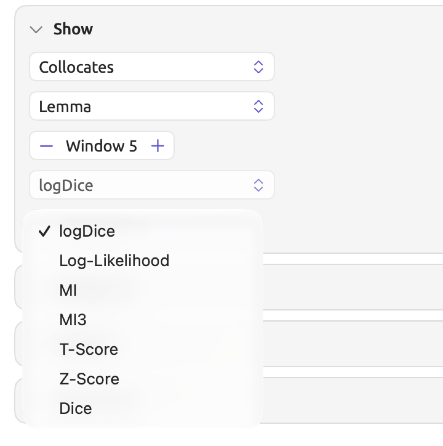
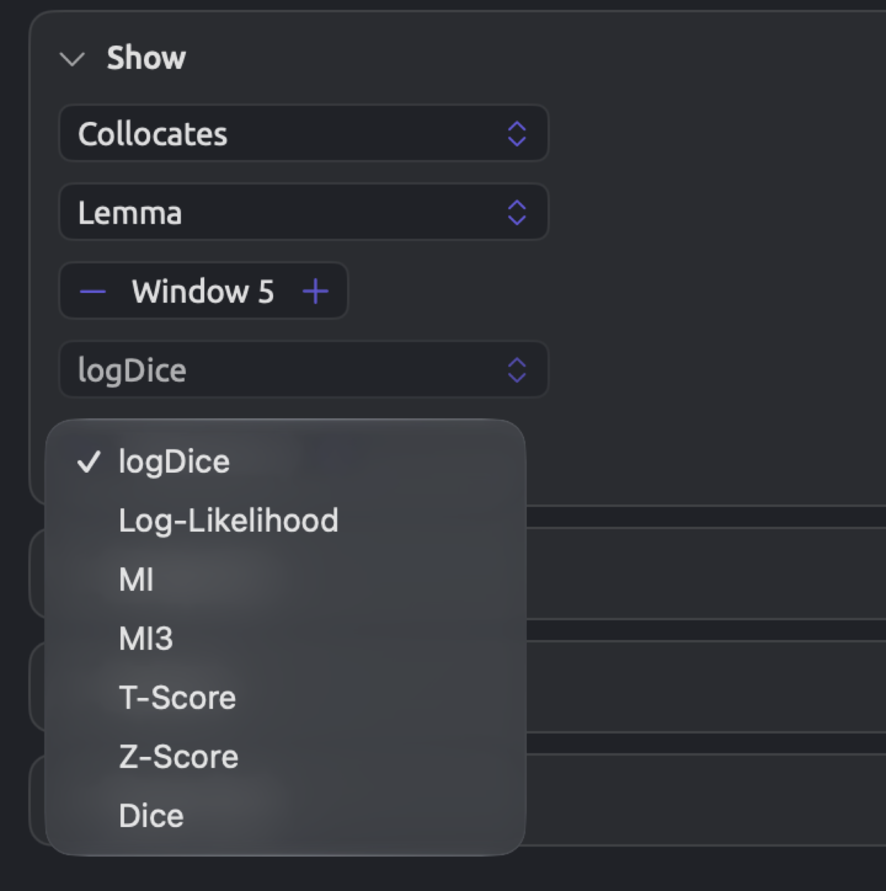
- In the Collocates result of a query, you can choose any of the seven available scores in the menu showing logDice, namely logDice, Log-Likelihood, MI, MI3, T-Score, Z-Score, and Dice, shown with two decimals. By default, the score is logDice; the window ranges from 1 to 10 and starts at 5; punctuation is ignored, and stopwords count as collocates. Minimum ranges from 1 to 50, initially set to 3, and the list shows up to 200 collocates.
- The scores used in word sketches, Code Sketch, and the list of Sketch Space are frequency and logDice only. In a word sketch, refers to the total number of relations of this kind. In a Sketch Space cell, stands for the total number of relations of this kind under that code. Under Code Sketch, refers to the count of relations of all kinds found inside passages coded by this code. refers to the frequency of the partner in its word class (see logDice in Chapter 12, Word Sketch).
Windows always end at the end of a sentence in both the facet and queries. Windows are otherwise counted in different manners between the facet and queries, which means that the same pair may receive slightly different scores in each according to the same measure. logDice is the safest score when comparing lists from two texts with different lengths ( does not factor into logDice).
Keyword and profile scores
Keyword lists compare your target with a reference. Passages Like a Code employs the same scoring technique to compare the words found inside versus outside the codings of one code. In the score calculation formulas, and represent occurrences of a word within each side, while and are the word counts of each side. and refer to the expected counts. In Passages Like a Code, stopwords are ignored during scoring calculations.
| Score | Where | Formula | Values and reading |
|---|---|---|---|
| Log-likelihood | The Log-Likelihood column of keywords; the weights of a profile | 0 or more. Keyword lists keep words at LL ≥ 3.84, LL ≥ 6.63, or LL ≥ 10.83. Common words reach high values easily | |
| Log ratio | The Log Ratio column of keywords; the rules of a profile | No limit; 0 means the same rate, 1 twice as often, −1 half as often. A size of at least 1 either way is a common minimum for a difference worth noticing | |
| Score | Lists sorted by Score | No limit. Compare scores only within one list |
The log-likelihood of hope (see Expected counts earlier in this chapter) is 5.34. The log ratio is
Therefore, the activists use hope almost 4 times as frequently as the skeptics. Raw rates of 30.0 and 6.7 occurrences per 10,000 words respectively yield a ratio of 4.5. Adding 0.5 to each count pulls the log ratio toward 0, particularly with lower counts.
Keyword lists consist of two lists. The Positive Keywords list consists of the words the target uses more often, while the Negative Keywords list consists of those it uses less often, with a negative log ratio. Only the words that reach the threshold and occur 3 times minimum on their own side, within the target for positive keywords and within the reference for negative keywords, enter the lists. Up to 200 words are shown for each, ranked based on log-likelihood. For further explanation on how the scores of the keyword list items work, see How the two scores are calculated in Chapter 16, Query Results and Statistics.
The Passages Like a Code profile is chosen from the words appearing at least 3 times within the codings with a log ratio of at least 1. The top-scoring 50 words by log-likelihood enter the profile along with their log-likelihood values as weights. For more information about how a code profile is formed, see How the profile is learned in Chapter 17, Query Patterns and Discovery.
In the score, to are the weights assigned to the different profile words that occur within a passage, each counted once, and is the total number of words within that particular passage. At least two different profile words should appear within a passage for it to be listed, except when a single word comprises the entire profile, in which case one profile word suffices. The total score of a nine-word sentence containing two profile words of weights 20 and 16 becomes .
Freeze Values converts the first 200 rows of a collocate or keyword list result into a frozen list; for keyword lists, only the Positive Keywords list is retained. All words maintain their scores from the result as weights. A query built on the list can then sort the matching passages by Score in the same way, requiring 2 distinct words of the list at minimum in a passage. See Freeze Values in Chapter 18, Using Query Results.
Measures in queries
Count, Compare, and Over Time display a selected measure out of five. Select the desired measure from the menu showing Hits (see Measures in Chapter 16, Query Results and Statistics).
| Measure | What it shows | Values |
|---|---|---|
| Hits | The number of hits | Whole number |
| Documents | The number of documents with at least one hit | 0 to the number of documents read |
| Per 10,000 Words | , pooled over the documents of the row | 0 or more |
| Coverage | The characters covered by at least one hit, divided by the characters of the documents of the row | 0% to 100% |
| Share | The row’s hits divided by all hits | 0% to 100%; the rows can add up to more than 100% when a hit has several values |
With a document-level key such as “Stance”, the words and characters of a row are those contained within the documents with that value. With any other key, such as Code, they are the words and characters contained within all documents that were read by the current query.
With a key set to Position in Document, which is set by Over Time whenever the key is left blank, a strip will be drawn depicting the hits in each document, along with two figures above the strips pertaining to how these hits are distributed across documents (see Where hits fall in each document in Chapter 16, Query Results and Statistics). If the key refers to a date field or Media Time, Over Time draws the chosen measure as a line chart.
| Figure | What it shows | Values |
|---|---|---|
| Range | Documents with at least one hit, out of all documents read, as in 5 / 6 | 0 to all documents |
| DP | 0 to just under 1 |
The DP measure is determined by the number of hits () and the size () of each document , with totals and . This size is measured either in words or in characters if the query does not count words. A DP value of 0 indicates that the hits were distributed in exact proportion to the sizes of the documents. The highest value of DP that can ever occur is 1 minus the smallest document’s proportion of the whole text. Two equally sized documents, where all hits occur in only one of them, would achieve , the highest value two such documents allow.
Coding statistics
The views of the shelf count original documents only, so a coding copied onto a translation counts once. What the views count in Chapter 13, Analyzing Codes explains the other rules.
| Statistic | Where | What it measures | Values |
|---|---|---|---|
| Segments | Codebook; Code Stats in the shelf; the count beside each code in the Code Stats facet | The codings of a code. In the Code Stats facet, a coded memo counts too, and its passage takes part in coverage and φ | Whole number |
| Documents | Codebook; Code Stats in the shelf | The documents with at least one coding of the code | 0 to the documents in the scope |
| Coverage | Codebook; Code Stats in the shelf and in the facet | The characters a code covers, overlaps counted once, divided by the characters of the scope or document | 0% to 100% |
| CO-OCCURS WITH | Codebook | The overlapping pairs of segments of this code and each other code | Whole number |
| Overlaps | Pairs in Relations in the shelf; the tooltip of a cell in Grid | The overlapping pairs of segments of two codes in the scope | Whole number |
| Code Matrix cells | Code Matrix in the shelf | The segments of each code in each document; with Group columns by, the codings, documents, or covered characters of each group, as chosen with the first switch | Counts; with Group columns by, counts (#) or percentages (%) |
| φ | Co-occurrences in the Code Stats facet; Relations in the shelf | How strongly two codes overlap, measured in characters (in Relations, the characters of every document in the scope) | 0 to 1 |
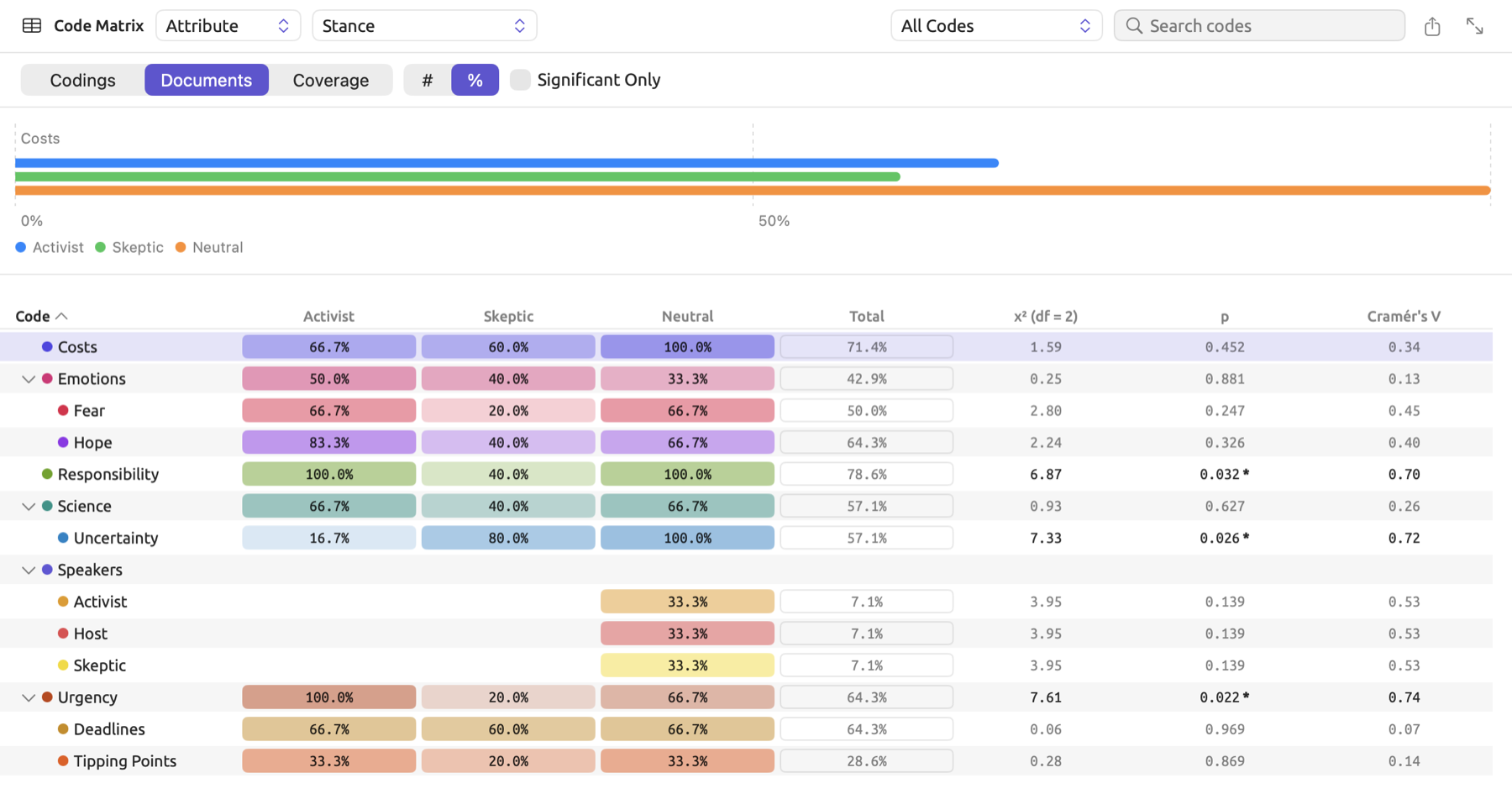
In the Code Matrix with %, each cell value is calculated relative to its own column group’s base. You may see the base value of a column group by hovering the mouse pointer over the group’s heading. Codings will become percentages of the group’s total codings; Documents, percentages of the group’s documents that have the code; Coverage, the percentage of the group’s characters the code covers (see Grouping the columns in Chapter 13, Analyzing Codes).
φ for overlapping codes
The Co-occurrences section of the Code Stats facet lists every pair of codes having overlapping segments in the document, ranked with the highest φ value first. Each row shows φ itself and the number of overlapping pairs of segments, and any pair having a p-value less than 0.05 receives a * after its names. Co-occurrences in a document in Chapter 13, Analyzing Codes works through the calculation. When computing φ in the Relations view of the shelf, the formula works the same way and uses the characters of all documents in the scope.
The table underlying φ assumes that every single character in the document represents one observation. “Running Out of Time” consists of roughly 5,000 characters. For simplicity’s sake, this example assumes “Costs” takes up 250 characters, “Responsibility” 200, while both share 100 characters:
| In “Responsibility” | Not in “Responsibility” | Total | |
|---|---|---|---|
| In “Costs” | 100 | 150 | 250 |
| Not in “Costs” | 100 | 4,650 | 4,750 |
| Total | 200 | 4,800 | 5,000 |
The expected overlap is characters. The codes have ten times as much overlap as that. The other three cells expect 240, 190, and 4,560, so every cell lies 90 from its expected count:
To calculate φ, divide χ² by and take the square root. Here, represents how many characters were in the document.
The p-value was derived from the chi-square distribution with one degree of freedom, giving you a p far below 0.001.
With thousands of characters being your observations, the p-value will tend to be tiny for almost any overlap, and neighboring characters are hardly independent. Within a long document, nearly every pair has a *. You thus need to evaluate pairs based on their φ, not their *. This becomes true to an even greater extent in Relations, since the characters of all the documents in the scope get pooled together.
φ has no sign. Should one pair overlap less often than chance predicts, you’d still end up getting a φ above 0, and often a *. If “Costs” and “Responsibility” had shared only 2 characters, just one-fifth of the 10 expected, their φ would come out at roughly 0.04, with a *. To distinguish between attraction and avoidance, check the observed overlap versus the expected overlap. The CSV export provides you with the former under the Characters column. Expected overlap is simply the characters of one code multiplied by the characters of the other code, divided by the characters of the document.
Tests
| Test | Where | Reported as | Effect size | Explained in |
|---|---|---|---|---|
| Mann-Whitney U | Compare, Rank Test on Rates, two groups | U, p | r | Chapter 16, Query Results and Statistics |
| Kruskal-Wallis H | Compare, Rank Test on Rates, three or more groups | H, df, p | ε² | Chapter 16, Query Results and Statistics |
| Chi-square on counts | Compare, Chi-Square on Counts | χ², df, p | Cramér’s V | Chapter 16, Query Results and Statistics |
| Fisher’s exact test, two-sided | Compare, Presence Test, two groups; Code Matrix with two groups | χ², df, p in Compare, where p is Fisher’s and χ² is given for comparison; p (Fisher) in the Code Matrix | φ in Compare; Cramér’s V in the Code Matrix | Chapter 16, Query Results and Statistics; Chapter 13, Analyzing Codes |
| Chi-square on presence | Compare, Presence Test, three or more groups; Code Matrix with three or more groups | χ², df, p | Cramér’s V | Chapter 16, Query Results and Statistics; Chapter 13, Analyzing Codes |
| Chi-square on a table | Compare with two Group By keys | χ², df, p | Cramér’s V | Chapter 16, Query Results and Statistics |
| Chi-square on characters | Co-occurrences in the Code Stats facet; Relations in the shelf | * when p < 0.05; p in the CSV export of Co-occurrences and in Relations | φ | Chapter 13, Analyzing Codes |
| Fisher’s exact test, one-sided | Sketch Space; the Multimode mode of the Word Sketch | * | None | Chapter 12, Word Sketch; Chapter 14, Sketch Space |
| Log-likelihood threshold | Keywords | Log-Likelihood | Log ratio | Chapter 16, Query Results and Statistics |
The statistics reported by the tests answer these questions:
| Statistic | What it asks | Values |
|---|---|---|
| U | Do the documents of one group tend to have higher rates than those of the other? | 0 to . LemmaLoom reports the smaller of the two possible values, so a smaller U means a clearer separation; 0 means every document of one group is ahead of every document of the other |
| H | The same question for three or more groups | 0 or more; larger means the groups’ average ranks lie farther apart |
| χ² | Do the counts of the table lie farther from their expected counts than chance would allow? | 0 or more; larger means a bigger departure. In Fisher’s exact test, read p and treat χ² as a comparison only |
| G² | Does a word’s count differ between target and reference by more than chance would allow? | 0 or more; compared with the value in the menu showing LL ≥ 3.84 |
Choosing a test in Chapter 16, Query Results and Statistics sets out which test should be used for each individual question.
Compare, the Code Matrix, and Sketch Space are three different tools within LemmaLoom that conduct tests. The following describes what is tested by each tool:
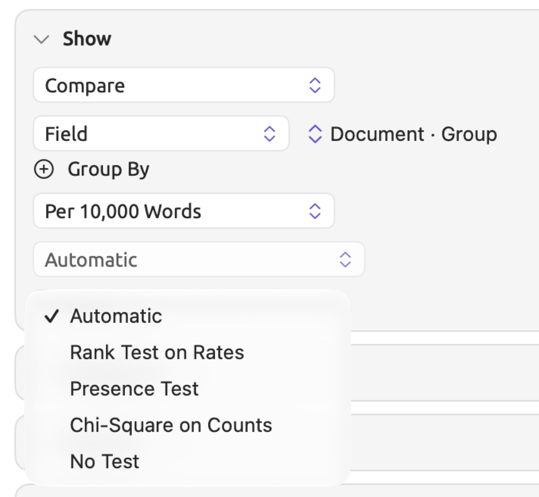
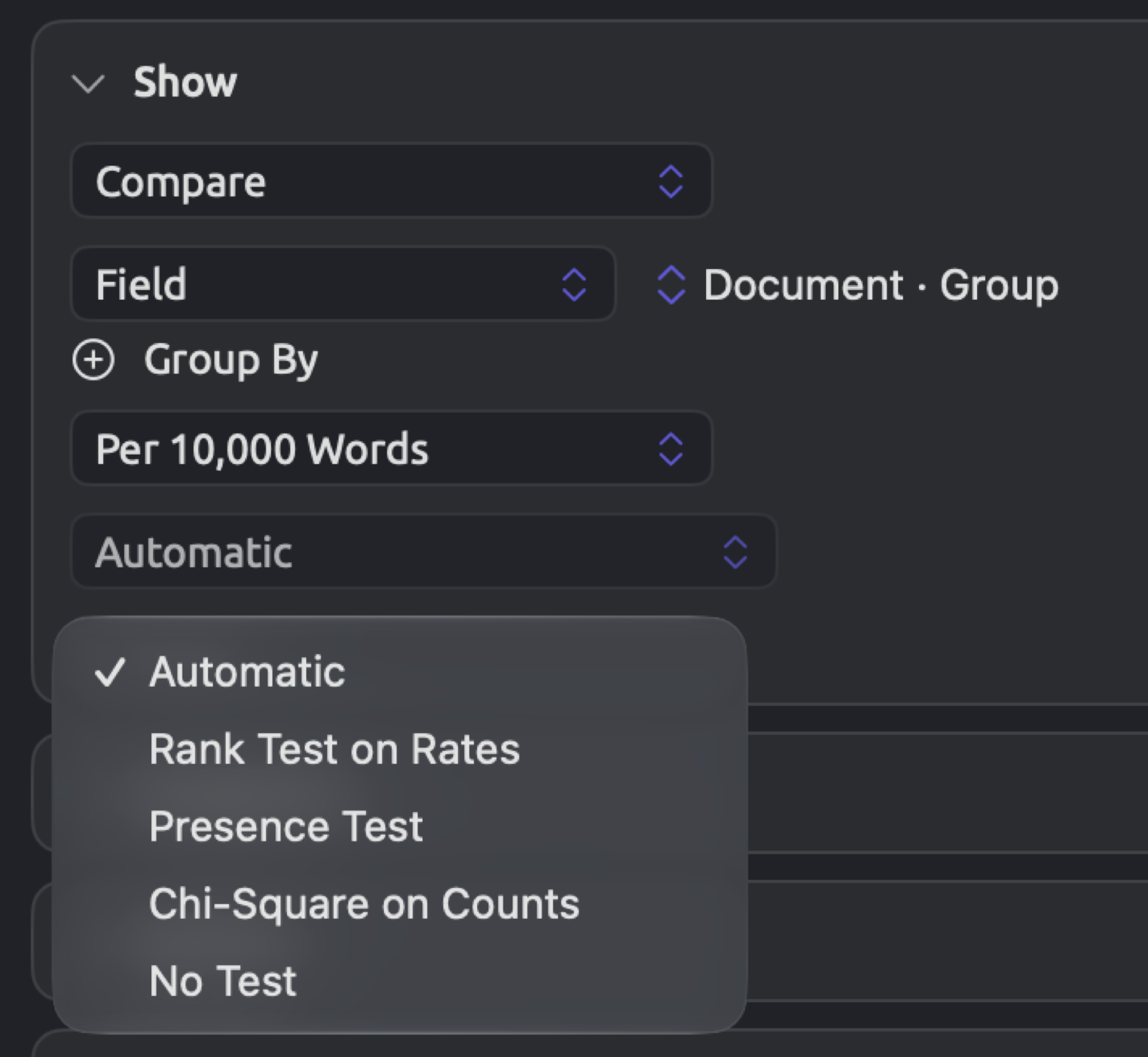
- Compare tests documents. When using one Group By key, Compare tests only when the key is document-level, such as attributes like “Stance” or the document’s Group itself. Tests available in the menu showing Automatic include Automatic, Rank Test on Rates, Presence Test, Chi-Square on Counts, and No Test. If the measure equals Documents, Automatic chooses the presence test; otherwise, the rank test is chosen instead.
- The rank test measures each document’s rate per 10,000 words or per 10,000 characters if the query did not count words, whatever the rows show. This is shown in more detail in Running a comparison in Chapter 16, Query Results and Statistics. All the documents get counted regardless of hits; documents without hits have a rate of 0. The presence test counts how many documents have hits vs no hits, which means you must have at least one of each type for the test to run.
- Should you specify two Group By keys, Compare will analyze the table formed by Group By rather than individual documents. In that scenario, Automatic will perform chi-square testing only when Find is Documents or any other unit that belongs to the Library group, while Chi-Square on Counts and Presence Test will run the test against table cells. Rank Test on Rates works with one key only.
- The Code Matrix applies the hypothesis tests to each code separately, whatever the two switches show; specifically, the null hypothesis says that there is no difference between the shares of documents containing each particular code within each group. Groups with No value (or Ungrouped for document groups) are skipped over as part of testing, whereas Compare treats them as a group of their own. If a code is in all or none of the analyzed documents, its test cells display a dash.
- Sketch Space marks a cell with * only if it contains at least 3 relations, more than what would be expected. Moreover, this difference in frequency must be statistically significant enough that the p-value of the one-sided test is less than 0.05.
How significance is shown
Wherever LemmaLoom highlights significance, it uses the cutoff p < 0.05, with these differences in formatting for display:
- Compare prints the test line darker when p is below 0.05, and gray otherwise. It displays the statistic rounded to two decimal places, while displaying the p-value and effect size rounded to three decimal places. Any value of p smaller than 0.001 is displayed as p < 0.001.
- The Code Matrix darkens the test values associated with a particular code if they are significant (p < 0.05); additionally, a * is appended after the p-value. The statistic and Cramér’s V will both display their values to two decimal places, whereas p-values will display to three decimal places, except values smaller than 0.001, which display as < 0.001.
- Relations marks any cells which are significant within Grid (displayed via a * in the corner of the cell) and Pairs (displayed via a * after the p-value); p-values smaller than 0.05 are also printed darker in Pairs.
- The Code Stats facet adds a * after the names of a pair of codes.
- Sketch Space and the Multimode mode of the Word Sketch add a * next to the count within the grid cells. Beneath the grid is a line indicating what this mark means.
In keyword lists, any words not reaching the log-likelihood chosen in the menu showing LL ≥ 3.84 are hidden.
Small groups
When there are only a few documents involved, the rank test won’t return a low p-value regardless of how large the difference may appear. Its lowest p-value will occur when every document in one group ranks higher than every document in the other group:
| Documents in the two groups | Smallest p | Largest r |
|---|---|---|
| 2 and 2 | 0.121 | 0.775 |
| 3 and 2 | 0.083 | 0.775 |
| 4 and 2 | 0.064 | 0.756 |
| 4 and 3 | 0.034 | 0.802 |
| 6 and 4 | 0.011 | 0.809 |
| 7 and 4 | 0.008 | 0.798 |
| 10 and 10 | < 0.001 | 0.845 |
The “Skeptics” set contains three printed documents (“The Models Keep Missing”, “Net Zero Will Cost You”, and “Science Is Never Settled”) and two online documents (“Let’s Not Panic” and “Who Pays for the Transition”). Without a shared rate among these documents, a rank test by Group within this set cannot give a p-value lower than 0.083. A gray test line there is to be expected merely from the number of documents contained within the set, even if skeptics in print and online media vary considerably in terms of the frequency of hedges. The numbers presented in the table assume no tied rates between any documents; ties can lower p and raise r considerably. With four documents without hits against two documents with different rates, for example, p is 0.028 and r is 0.894.
The maximum r value also depends on the sizes of the two groups. Without tied rates, the value of r never reaches 0.87, and it stays far lower when the two groups differ greatly in size.