Analyzing Codes
Once you have coded enough passages in your documents, you can take a look at the distribution of codes, and the ways in which groups of documents may use your codes differently. LemmaLoom’s views count occurrences of each code and how much text it covers. One view displays the location of each code occurrence in each document. Another view shows how different codes co-occur.
Views are available for single documents in the Coding tab of the inspector, and for projects, sets, and tags in the project shelf (see The project shelf in Chapter 3, Projects and Documents). Additional explanations on setting up codes and coding passages are in Chapter 7, Coding.
The following demonstrations use LemmaLoom’s example project entitled “Climate Debate” (File ▸ Import ▸ Example Project). LemmaLoom adds “Climate Debate” in the language of the interface, complete with its documents indexed and all codings pre-applied. The “Climate Debate” example project uses the codes “Urgency” (subcodes “Tipping Points” and “Deadlines”), “Science” (“Uncertainty”), “Costs”, “Responsibility”, and “Emotions” (“Fear” and “Hope”). Additionally, “Radio Debate” includes “Speakers” (with the speaker codes “Host”, “Activist”, and “Skeptic” as subcodes), which groups the speaker codes, so that the project’s Code Stats lists 13 codes. The document sets include “Activists” containing the six activist documents and “Skeptics” containing the five skeptic documents.
The counts of segments, documents, and overlaps below refer specifically to the example project provided by LemmaLoom. The character counts in the examples are made up for demonstrative purposes and kept round, making the calculations simple to track. The example project itself therefore shows different coverages and values of φ.
Key terms
- A coding refers to one application of a code to a passage of text. If a passage is coded with two codes, it has two codings.
- A coded segment, or segment, refers to the passage covered by one coding, and in the counts of the views is synonymous with coding.
- The scope of a view is the documents it covers, whether the active document in the inspector, or a project, a set, or a tag in the shelf.
- The coverage of a code is the proportion of characters within the scope’s text spanned by the code’s segments, expressed as a percentage.
- Two codes overlap, or co-occur, whenever a segment of one shares at least one character with a segment of the other within the same document.
- A code is present in a document that has at least one segment of that code.
- An attribute is a property attached to a code, such as “Intensity” attached to “Fear”. It holds values in every coding of the code to which the attribute applies, which are used by the attribute breakdowns and the filter of the Codings view; Group columns by in the Code Matrix instead groups columns according to document attributes, e.g., “Stance”.
- φ (phi coefficient) is a normalized measure of association, ranging between 0 and 1, representing the extent to which two codes co-occur compared with what one would expect through pure chance alone.
- Similar to the phi coefficient, and on the same scale, is Cramér’s V, but rather than measuring overlap between codes, it compares proportions of documents containing a code within each group.
- The p-value is a probability measure for testing how unexpected a result would be if due solely to randomness; the smaller it is, the more unexpected the result.
Choosing a view
Choose a view depending on what interests you most:
| To see | Use | Scope |
|---|---|---|
| How often each code is used, and how much text it covers | Code Stats | One document, or a project, set, or tag |
| The order in which the codes come in a document | Portrait | One document |
| Which codes overlap in a document, and how strongly | Co-occurrences in Code Stats | One document |
| Every coded passage, with its attribute values | Codings | One document, or a project, set, or tag |
| How the values of a code’s attribute are spread | Attribute Breakdowns in Code Stats | One document, or a project, set, or tag |
| Which documents use which codes | Code Matrix | A project, set, or tag |
| Whether groups of documents, such as activists and skeptics, use a code in different shares of their documents | Code Matrix with Group columns by | A project, set, or tag |
| Which codes overlap across many documents, and how strongly | Relations | A project, set, or tag |
| How one word’s grammatical partners differ between codes | Code Sketch, or Coding in the Word Sketch view | One document, or a project, set, or tag |
To see rates of codings per 10,000 words, or to test rate comparisons of single documents, use a query with the Show option set to Compare (see Comparing groups in Chapter 16, Query Results and Statistics).
What the views count
- Code views in the project shelf count only original documents. Translated documents hold copies of their originals’ codings (see Codings in translations in Chapter 7, Coding), and counting them would count each coding twice. The facets of the inspector count the active document, so when looking at “Running Out of Time (German)”, its copied codings will appear.
- The Codes and Code Stats facets will consider coded memos as a coding of their codes (see Coded memos in Chapter 7, Coding), whereas the Portrait facet, attribute breakdowns, and code views in the shelf only consider actual codings.
- Each code is considered separately. Thus, for the code “Urgency” in the example project, only passages that were actually coded as “Urgency” itself contribute to the numbers. “Tipping Points” and “Deadlines” count separately as subcodes. In reading the segments behind a number in the Codings view, however, you can add the subcodes (see The Codings view).
- Coverage measures characters, including spaces and line breaks. Characters within overlapping passages for the same code count once.
The Coding inspector
The Coding tab in the inspector displays the codes of the active document. Select View ▸ Inspector ▸ Coding (⌥⌘3), or click the tag icon on top of the inspector. Six buttons beneath the icon tabs switch between the six different facets within the Coding inspector, Codes, Codings, Links, Code Stats, Portrait, and Code Sketch.
The first three facets deal with codes, codings, and links respectively, which are detailed fully in The Coding inspector in Chapter 7, Coding. Counters appear in each of these facets.
- The Codes facet displays alongside each code its frequency of use within this particular document. When you click the export button next to Code System, the list of codes with these numbers will be exported as a CSV file.
- The Codings facet displays all the codings within this document in reading order, displaying their number inside its switch, e.g. Codings (13). Using Filter by code reduces this list to display only those codings belonging to a particular code.
- The Links facet displays all the links with an end within this document, under a heading that gives their number.
Code frequencies and coverage
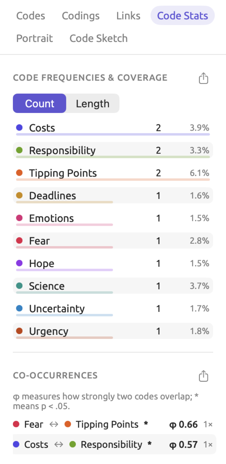
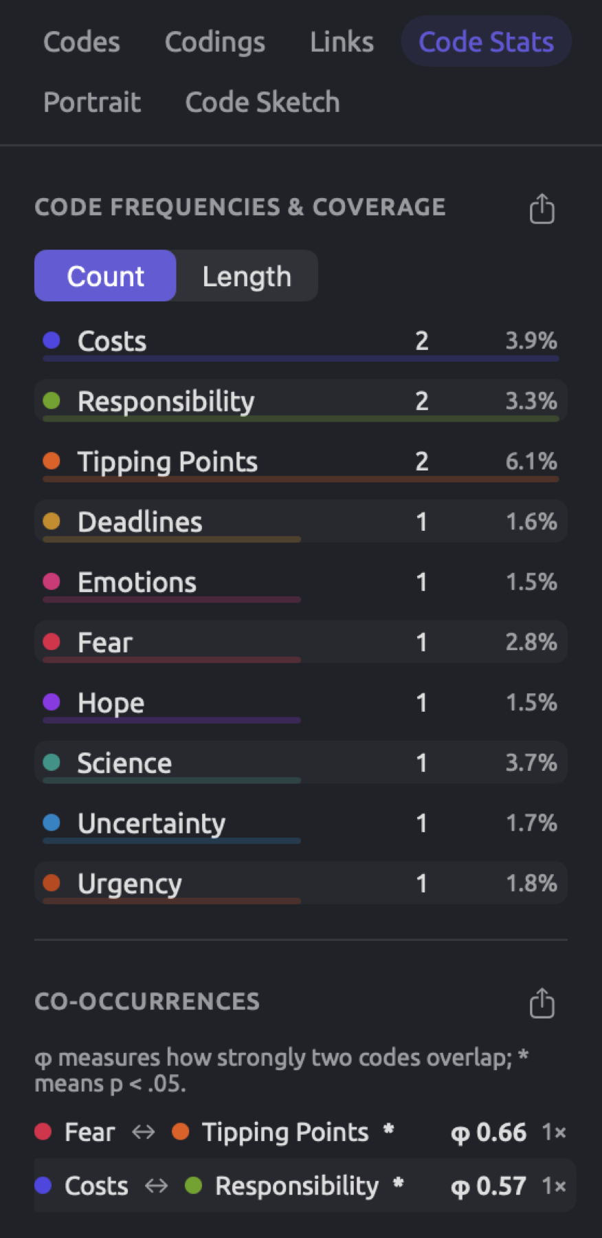
The Code Stats facet tracks the codings in the active document. In its first section, titled Code Frequencies & Coverage, every code found in the document is listed along with two numbers, which represent the total segments coded by that code in the document and the percentage of the document covered by that code, respectively. The figure shows the facet for “Running Out of Time”, one of the activist op-eds in “Climate Debate”.
To inspect the codes applied to a document:
- Open the document.
- Choose View ▸ Inspector ▸ Coding (⌥⌘3), and click Code Stats.
- Click Count or Length above the list.
Count ranks the codes according to their number of segments while Length ranks them by how many characters the segments span. The bar beneath each row corresponds with whichever ranking scheme is chosen, and the number for this measure is shown in a darker color than the other. Clicking on any row shows one of the code’s segments in the reader.
The formula for calculating coverage is the following:
refers to the number of characters contained in the segments belonging to the code in question, counting characters shared by overlapping segments of the same code just once. is the total number of characters in the document. Assume, as an example with round invented numbers, that the document “Running Out of Time” contains 5,000 characters, with its two “Tipping Points” segments covering 300 characters worth of the document. The row representing “Tipping Points” shows 2 for the number of segments. The coverage in this particular case is calculated as:
In reality, the row shows 6.1%, based on the real character counts of “Running Out of Time”. Looking at the coding of one text in Chapter 2, Getting Started contains another example showing coverage for overlapping segments.
Ranking by Count shows which codes are used the most often, whereas under Length a code with one lengthy segment may rank high. While “Science” occurs once in “Running Out of Time”, it covers 3.7% of the text. Conversely, “Responsibility” has two segments, but they cover only 3.3% of the document. Hence, “Responsibility” has a higher Count but a lower Length ranking compared to “Science”.
Co-occurrences in a document
Co-occurrences, the second section of Code Stats, lists every pair of codes that occur together anywhere within a document.
Every row includes the two codes linked with a bi-directional arrow, followed by the φ coefficient, and the count of overlapping pairs of segments, e.g., 1×. A * after the code names indicates the p-value of the pair falls beneath 0.05. Rows sort in order of decreasing φ value.
For “Running Out of Time”, the row for “Tipping Points” and “Fear” displays *, φ 0.66, and 1×. The one “Fear” segment intersects with one of the two “Tipping Points” segments. φ quantifies the relationship based on how much text they share compared to chance, weighted by how much of the document each code covers.
The four counts
This measure considers every character within a document as one observation. An observation belongs to one of four cells depending on whether it belongs to both codes, “Fear” alone, “Tipping Points” alone, or to neither. For instance, let “Fear” account for 200 characters of “Running Out of Time” and “Tipping Points” for 300, with an overlap of 120:
| In Tipping Points | Not in Tipping Points | Total | |
|---|---|---|---|
| In Fear | 120 | 80 | 200 |
| Not in Fear | 180 | 4,620 | 4,800 |
| Total | 300 | 4,700 | 5,000 |
“Fear” alone accounts for characters, while “Tipping Points” alone accounts for characters. The rest of the 5,000 characters, 4,620 of them, carry neither code.
Expected overlap
Suppose that the two codes were uncorrelated, meaning that if you knew where you coded “Tipping Points”, then you could not predict anything about where you coded “Fear”. In other words, the “Tipping Points” code would cover the same proportion of characters within “Fear” that it does of the whole document, 300/5,000 or 6%, and 6% of the 200 characters in “Fear” is 12. That’s the expected count of characters in the intersection of the two codes (the shared cell). For each cell in a contingency table like this, you calculate the expected count with the following formula.
In this context, stands for the expected number within a cell, for the total number of counts in its row, for the total number of counts in its column, and for the number of characters in the document. Hence, the expected number within the “Tipping Points” and “Fear” cell would be . Other expected numbers would be “Fear” alone expecting 188 characters, “Tipping Points” alone expecting 288 characters, and neither expecting 4,512 characters. There are 120 shared characters between the two codes, 10 times higher than the expected 12.
Chi-square
The chi-square statistic () adds up the difference between each observed cell count and its expected count.
The observed cell count is denoted by ; the expected cell count is represented by . Summation notation () here refers to “add up the following for every cell”. Squaring ensures that differences above and below expectation both contribute positively to the sum. Dividing by makes low counts matter more relative to high counts.
In a two-by-two table, each count deviates from its respective expected count by the same amount, here 108 (, , etc.), and . Here’s how is calculated:
Almost all of stems from the shared cell, with 120 characters versus the expected 12 characters.
Phi
The measure χ² increases linearly with the length of the document. Doubling all counts will double χ². φ eliminates this dependency:
In the case of “Tipping Points” and “Fear”:
This value of φ is determined from the round counts. From the actual character counts in “Running Out of Time”, the row of “Tipping Points” and “Fear” lists φ 0.66. φ equals 0 if two codes overlap exactly as much as expected and equals 1 if both codes span identical sets of characters.
Any short code completely encompassed by a larger code results in φ values strictly smaller than 1. If the entire 200 characters of “Fear” had also received the “Tipping Points” code, the four cells would contain 200, 0, 100, and 4,700. Such observations would produce a χ² statistic near 3,264, leading to due to the 100 additional “Tipping Points” characters not contained within “Fear”.
In LemmaLoom, φ can never take negative values. Thus, pairs with unexpectedly low co-occurrences receive positive values. In general, whenever codes overlap at all, they overlap more than expected because code coverage in every document tends to be low. To check whether two codes overlap less than expected, compute their expected overlap by multiplying the number of characters in each code together and dividing this product by the total number of characters in the document. Then compare this expected value against the observed number of overlapping characters found in the Characters column of the Co-occurrences CSV file. Each code’s number of characters can be located in the Characters column of the Code Frequencies & Coverage CSV file, while individual document lengths reside in the Characters field of the Text inspector.
The p-value and the *
Two codes placed randomly would overlap somewhat more or less than expected, so χ² would rarely equal exactly 0. A p-value is essentially the probability of χ² being at least as large as observed under conditions of no relation between the two codes. If p is 0.03, for instance, it means unrelated codes would produce a χ² at least that large about 3 times out of 100.
The χ² values that chance produces have a certain predictable form, the chi-square distribution. It varies based on the degrees of freedom; this term refers to the number of entries in the table free to vary upon specifying the marginal sums (totals in each column and row). In a 2 × 2 contingency table, there is one degree of freedom (the shared cell and the totals fix the other three cells), meaning chance would produce a χ² of 3.84 or greater 5 times in 100 tries. LemmaLoom calculates the probability based on the distribution and adds an asterisk to pairs whose probabilities are below 0.05, which is when χ² is above 3.84. In a spreadsheet, =CHISQ.DIST.RT(3.84,1) equals 0.05. Replace 3.84 and 1 with any χ² and number of degrees of freedom to get its probability.
Consider “Tipping Points” and “Fear”, with a χ² of 1,077; they lie way beyond 3.84, along with nearly every pair overlapping by more than a few words. Assume in this op-ed piece that you started the “Uncertainty” segment two words early, placing it partly within the “Tipping Points” segment before it. Here “Tipping Points” spans 300 characters and “Uncertainty” spans 100, overlapping by 12. The expected overlap is characters. The remaining three numbers in the cells differ by 6 from expectation (288 instead of 294, 88 instead of 94, 4,612 rather than 4,606):
=CHISQ.DIST.RT(6.51,1) gives p ≈ 0.011, hence an asterisk. Its φ is .
An asterisk is this easy to earn because the test treats each of the 5,000 characters separately as an observation. However, character occurrences are clearly interdependent; the shared characters come from your choice of one place where a segment starts. The p-value thus exaggerates significance. Understand the * as “overlap unlike chance”, which nearly always means more, and measure the strength of a pair using φ, which is 0.46 for “Tipping Points” and “Fear”, and 0.04 for “Tipping Points” and “Uncertainty”. A high φ indicates merely that you coded two topics in the same places.
Attribute breakdowns
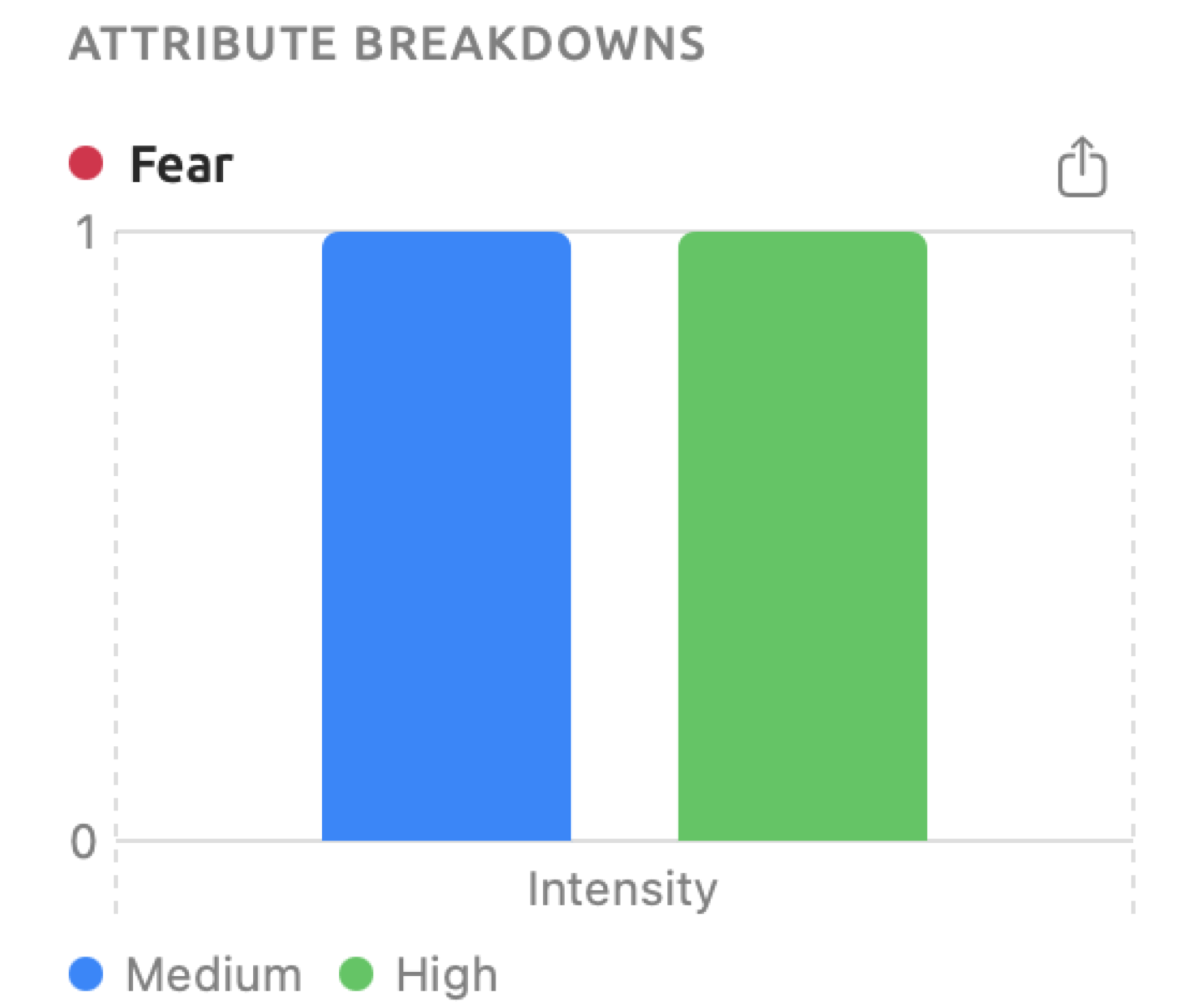
If a code possesses attributes (see Codes with attributes in Chapter 7, Coding), a new section named Attribute Breakdowns will show up at the end of the Code Stats facet. Each code that possesses attributes and was coded at least once in the active document receives its own chart showing how many of its codings hold each value. For the examples in this chapter, assume that “Fear” is a code whose attribute “Intensity” accepts the three options “Low”, “Medium”, and “High”.
Each attribute of the code has its own cluster, with one bar per value. A bar represents how many codings in total were made with the chosen attribute having that particular value. For a Picker (an attribute with a fixed list of choices), the order corresponds to the order of the options defined by the user in the attribute; numbers come in increasing order, and other values in alphabetical order, which puts dates in date order. Codings that don’t have any value in that attribute are shown last in an additional bar, labeled with a dash. Below the chart, there is a legend indicating which colors correspond to what values.
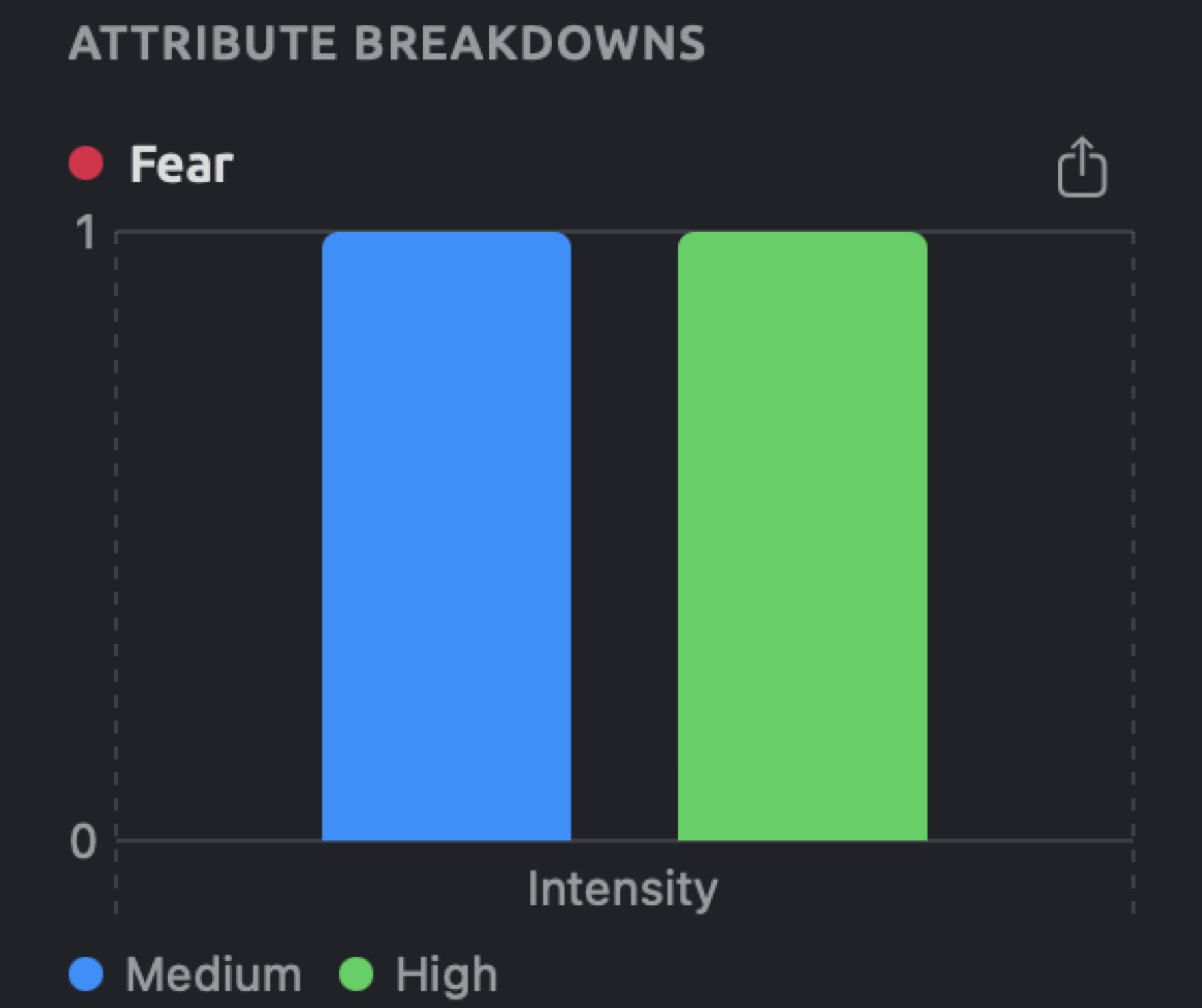
Assume that “Fear” appears twice in “Why We Block the Roads”, once having “Intensity” equal to “High”, and once having “Intensity” equal to “Medium”. Then the chart will feature two bars, one for each of these values in the order of the choices, with each bar being of height 1.
The Code Stats view of the shelf has the same section for projects, sets, and tags, and the codings that hold a particular value can be listed by filtering the Codings view (see Filtering by attribute values).
Portrait
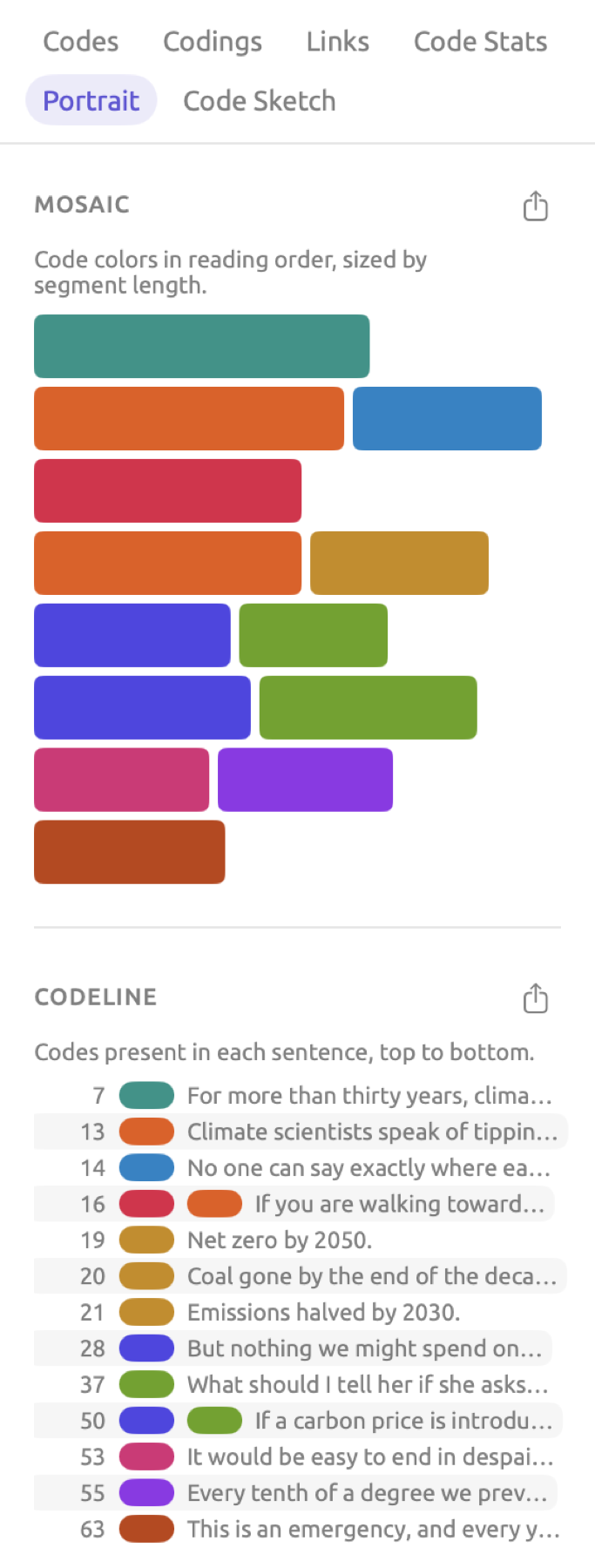
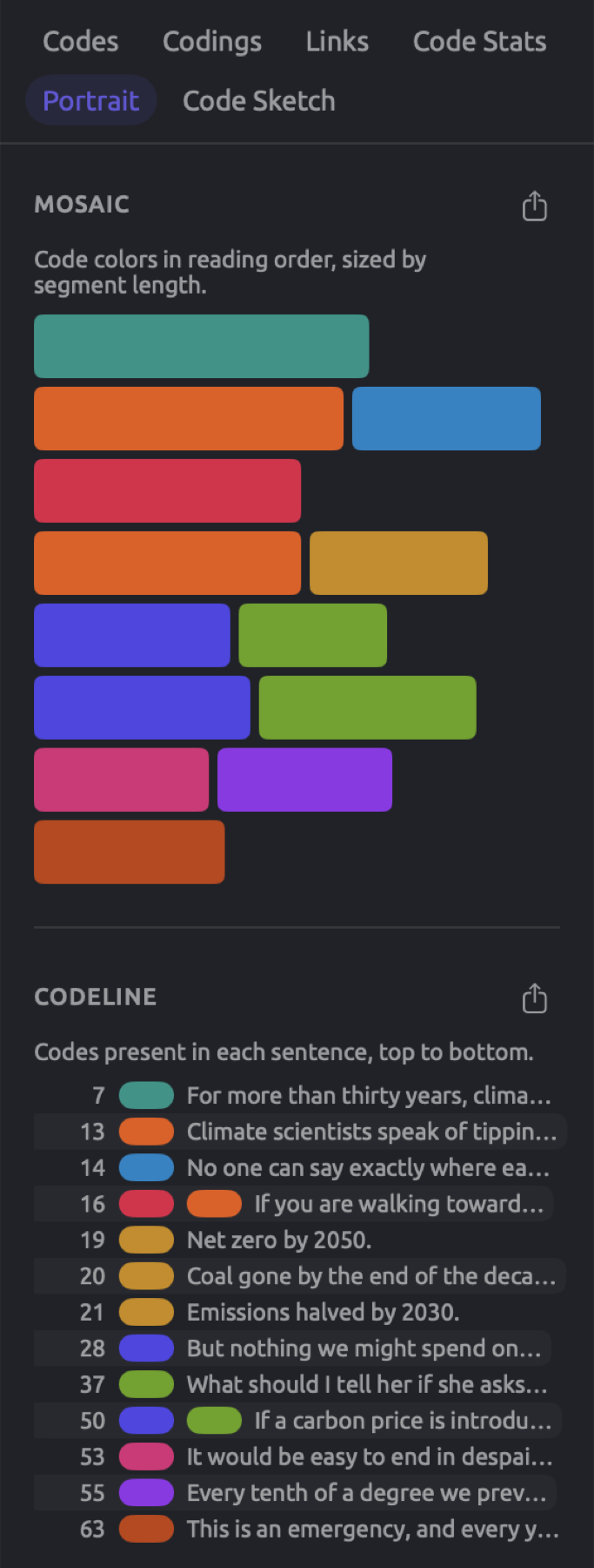
The Portrait facet provides a visualization of the coding applied to the active document in two ways. The first is Mosaic, which displays the order of occurrence of codes and the length of their segments. The second is Codeline, which provides a listing of the sentences that contain any of the applied codes in addition to displaying the codes of each sentence.
Mosaic
The Mosaic will display every coding present in the document as a tile; the tile’s color corresponds to the color of its code. The tiles are aligned according to the text’s natural reading order from left-to-right. Tiles will be displayed row-by-row. A tile’s width depends on how long the corresponding segment is; the longest segment gets the widest tile, and even the shortest segments get a small square. When you hover the mouse pointer over a tile, the name of the code and the text segment it contains become visible. Clicking on the tile will show its passage in the reader.
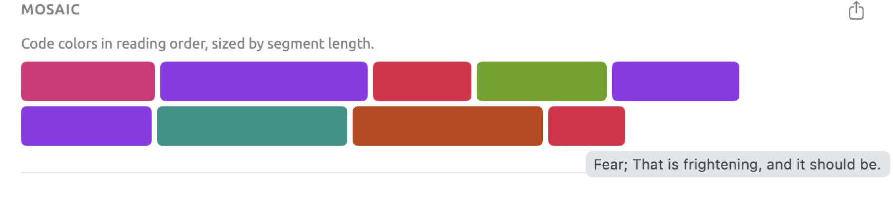
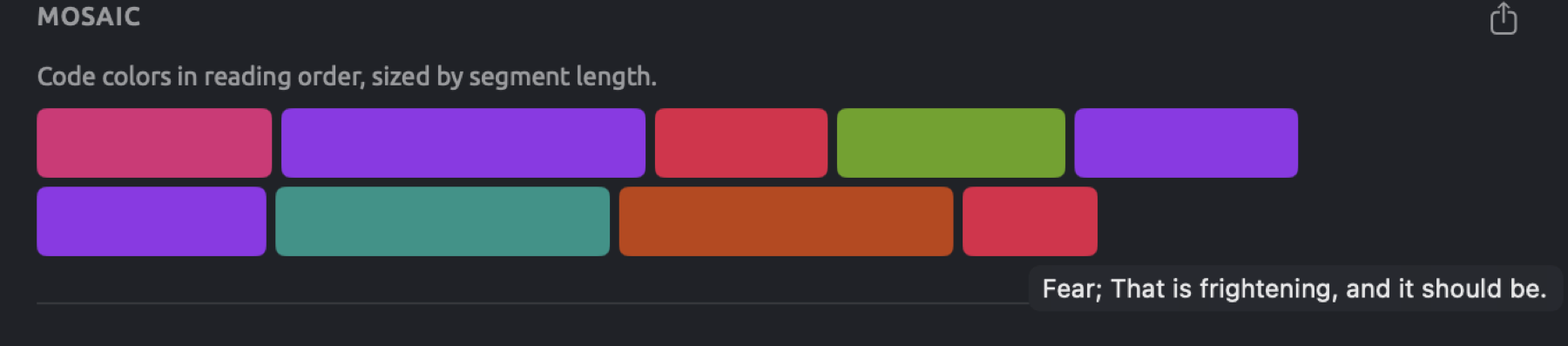
A run of tiles in one color shows a stretch on one theme; alternating colors mean the text moved back and forth, or that you gave the same passages several codes. Mosaics can be used to compare texts’ structures. Export the Mosaics for two texts and place the images next to one another for comparison. Each Mosaic scales its tiles to its own longest segment, so compare the order and mix of colors between Mosaics rather than tile sizes.
Codeline
Each row in the Codeline corresponds to one sentence touched by at least one coding, ordered as in the text. In each row are shown the sentence number, a colored bar for each coding touching the sentence, and the first few words of the sentence itself.
Hover the mouse pointer over a colored bar to display the code’s name. Click on the bar to view the coding within the reader. If the coding covers multiple sentences, it is shown separately for each sentence. When two codes touch the same sentence (two bars share a row), then both codes co-occur within that particular sentence; the Codeline thus displays the sentences behind a pair in Co-occurrences.
The Codeline uses information regarding the sentences found inside the document, which comes from indexing. Therefore, it remains blank until you index the document. In addition, indexing sentences works for English, German, and Chinese documents; in all other languages, the Codeline stays blank (see What is available without the analysis in Chapter 21, Analysis and Indexing). The Mosaic works in every document.
Code Sketch
Finally, the Code Sketch facet illustrates the grammatical associations of a particular word, grouped according to which codes cover occurrences of that word. This way, it tells you which words associate with climate in the segments coded “Urgency”, which words associate in the segments coded “Science”, etc. For a set, a tag, or the entire project, the Coding mode of the Word Sketch view of the shelf provides this exact visualization. To get additional info on Code Sketch, refer to Code Sketch in Chapter 12, Word Sketch. To compare a word across codes in a column-by-column manner, use Sketch Space (see Chapter 14, Sketch Space).
Code views for projects, sets, and tags
There are seven views of the project shelf for codes, namely Codebook, Codings, Memos, Links, Code Stats, Code Matrix, and Relations. When selecting any shelf view for the project from Project in the navigation sidebar, the selected shelf view opens in a tab of its own. When selecting any set or tag from the sidebar, its tab includes buttons for the various shelf views of the set or tag. The tab opens up to the view most recently visited for that set or tag, and the first time to the Codebook view. Should you need to keep a view of the whole project next to the reader, you can open it in the Codebook window using the Open in a window button at the right end of its header.
Each shelf view counts the original documents of its scope; the scope is every document of a project, the members of a set, or the documents having a particular tag. As you continue working, the numbers update accordingly.
You may learn further details about three of these shelf views in The Codebook view, The Memos view, and The Links view in Chapter 7, Coding. For a set or a tag, they show the following:
- The Codebook view shows every code of the project along with the number of segments coded by them in the scope’s documents, while the details of a selected code under USE IN THIS SCOPE and CO-OCCURS WITH refer solely to the scope’s documents.
- The Memos view lists the memos on the scope’s documents and their respective passages. Memos regarding a code or referring to the entire project, which could be part of a project imported from software compatible with the REFI-QDA format, are available exclusively in the Memos view of the project.
- The Links view lists all the links at least one endpoint of which lies inside the scope’s documents or their translations. A link and its copy in a translation count only once.
The Codings view
The Codings view gives you an overview of every coded passage in your selected scope. Each row contains details for one coding, including Document, Code, Segment, and Position. This means you are looking at your coding at the level of the individual passages themselves; you could check if your coding was consistent when dealing with a particular topic in various documents, or gather your quotes. The Segment column shows you the beginning portion of the coded passage itself, while the Position column tells you where exactly within the document this passage starts, counting characters from 0 at the start of the document. Rows are sorted alphabetically by document title, then by position, so each document’s rows follow reading order.
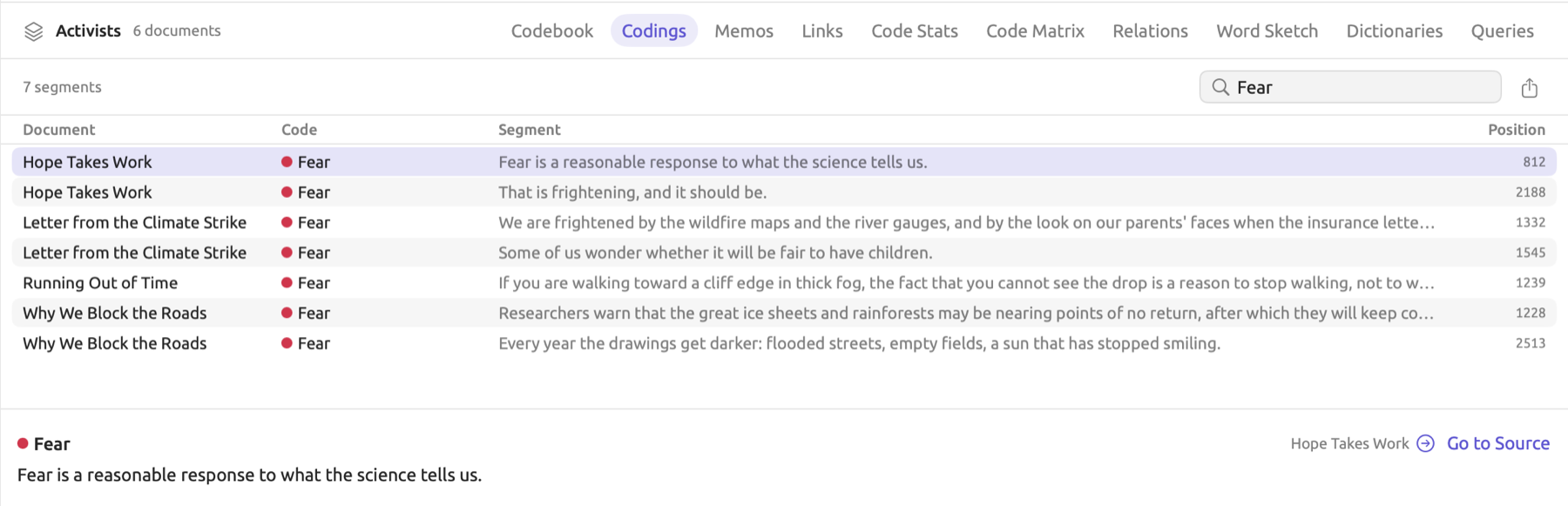
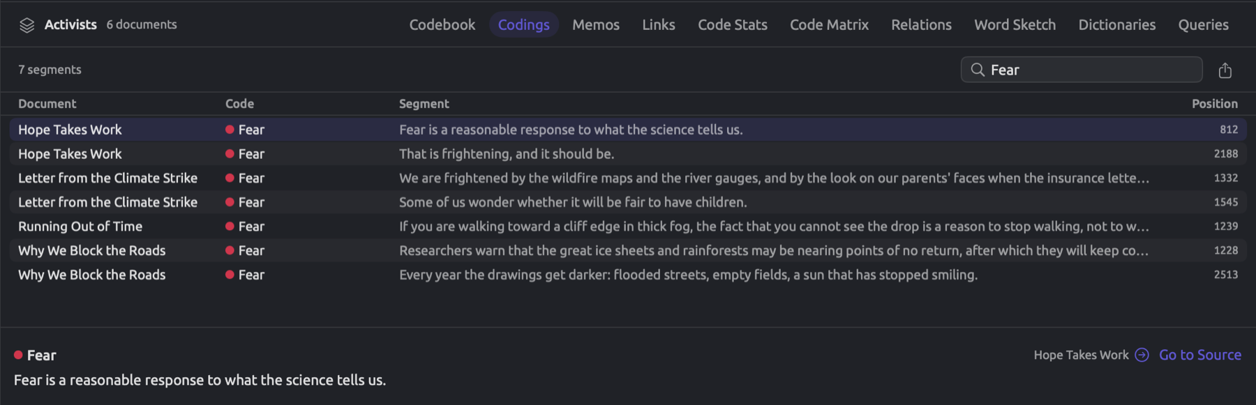
The number of rows shown in the header tells you how many segments are contained in your table. As an example, the “Activists” set has 54 segments. In addition to the number of segments, the header includes Search, the export button, and the filter button if any listed code has attributes.
- Clicking on one row allows you to explore the full segment, including its code, document, and attribute values, in the pane under the table. You can set or change its attribute values in the pane. To control the ratio between your table and your pane in the window, drag the border separating both.
- When double-clicking a row, hitting the Return key, or clicking Go to Source in the pane, the corresponding document opens up for you at that particular row’s segment.
- Right-clicking a row brings up the shortcut menu with the choices Go to Source, Change Code, and Delete Coding. To give the existing coding of a segment another code, click on Change Code (see The Codings facet in Chapter 7, Coding); either change is reversible with Edit ▸ Undo (⌘Z).
- Type in some text in Search to keep the rows that contain that text in any of their fields. These fields consist of the code name field, the coded text field, and the document title field.
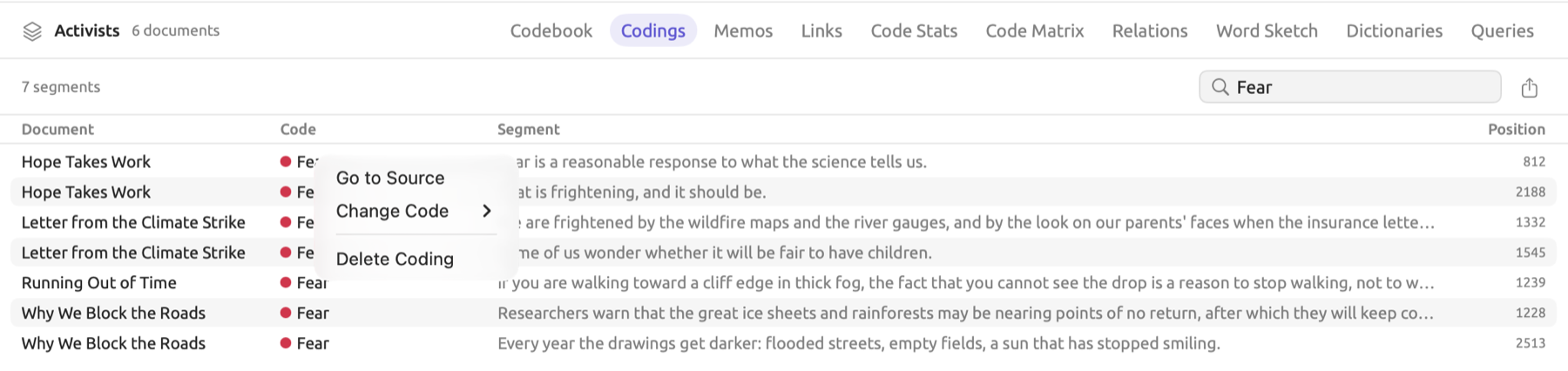
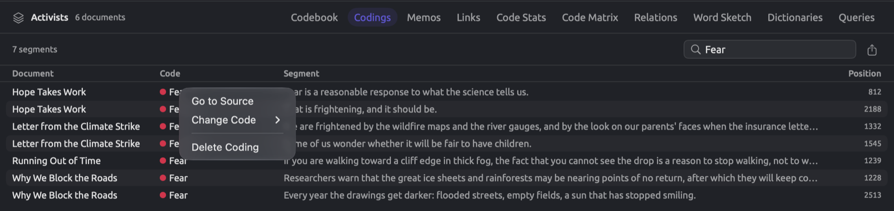
Because Search will check the coded text field and the document title field, entering “Hope” into Search within the “Activists” set would also show you every segment of “Hope Takes Work”. For viewing exclusively those segments assigned to one particular code, open them from another view, as described below.
The segments behind a number
The other code views can also reveal their underlying passages in the Codings view. This can be done by double-clicking any bar or row in Code Stats, any cell in Code Matrix, or any cell or pair in Relations; or right-clicking any row, cell, or pair, and choosing Show Codings from the resulting shortcut menu. Upon opening Codings, the view loads the codings behind the number you chose. Its header tells you which segments were loaded. For instance, in “Climate Debate”, the header reads Urgency · Activist for all “Urgency” codings applied to the activist texts. Similarly, the Show Codings option in the Codebook operates the same way as described earlier (please review The Codebook view in Chapter 7, Coding).
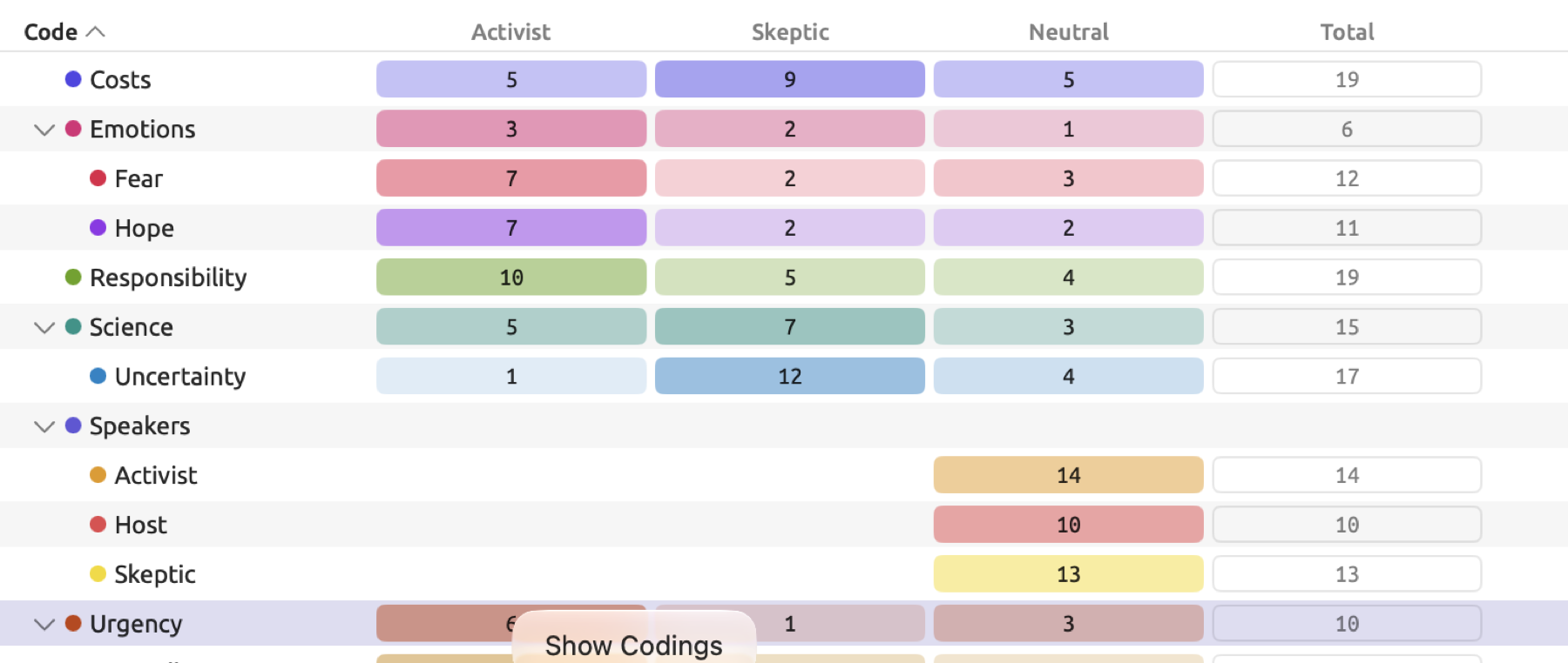
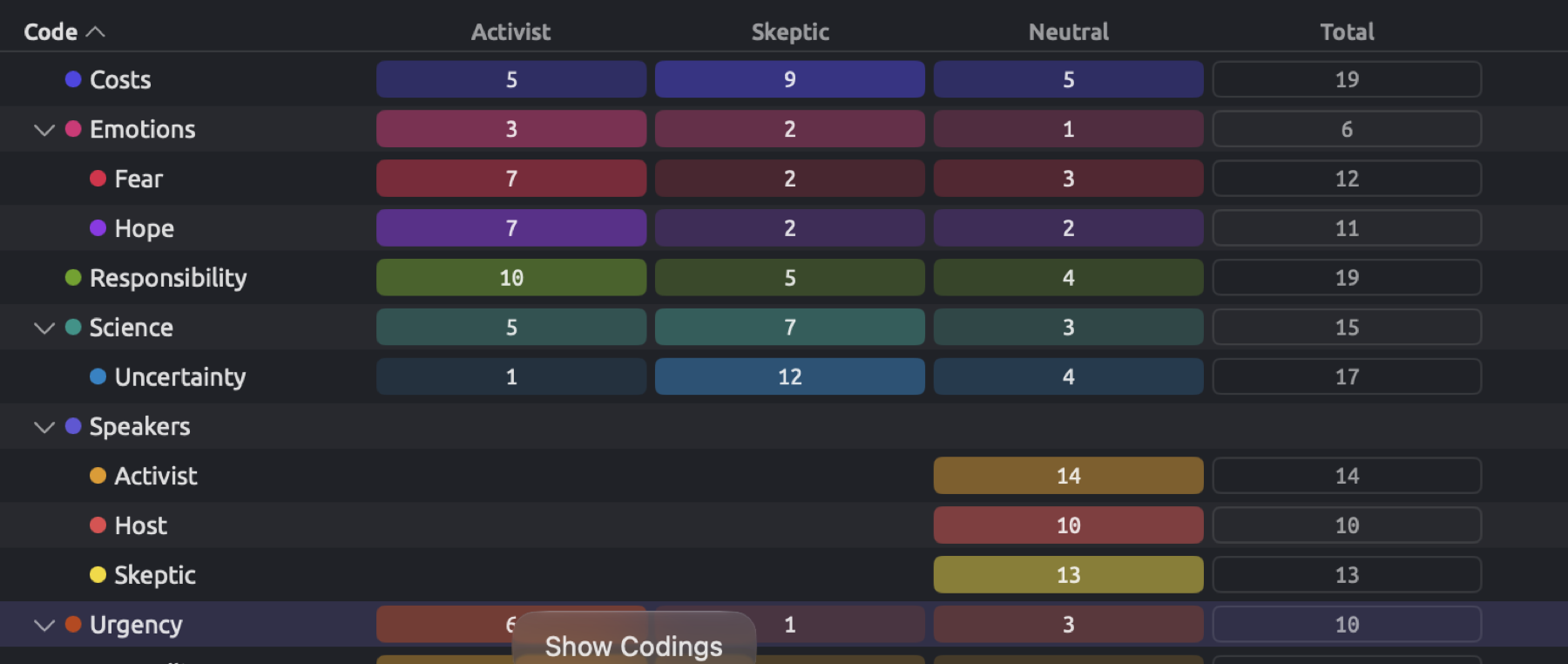
Numbers here count the occurrences of just the displayed code while its subcodes are ignored. Including the latter can be achieved by checking the box labeled Include Subcodes found adjacent to the code name. The No subcodes tooltip displays alongside the disabled Include Subcodes box when the code has no subcodes. The Search field and the attribute filter narrow down the results further. The × button (Remove filter) found adjacent to the code name will show all codings again, as does opening Codings through any other means.


Filtering by attribute values
If a code in the list possesses attributes, the filter button, represented as a funnel inside a circle, will appear next to Search. The filter limits your results to those codings having attribute values satisfying a particular condition, e.g., the strongest fears in the activists’ texts. Assuming you had an “Intensity” on “Fear”, filtering for “Intensity” is any of “High” in the “Activists” set leaves you with only 3 out of 7 “Fear” codings in total; hence the count becomes 3 segments.


To filter your segments by an attribute:
- Open the Codings view of the project, a set, or a tag.
- Click the filter button.
- In the popover’s first menu, which reads None, choose the attribute.
- In the menu beside it, choose a comparison, such as is any of.
- Set the value. For a Picker, click the button below, which reads None, and check a choice.
The header names the filter (e.g., Intensity is any of High), with the funnel appearing filled until the filter is deactivated. Clicking on the × icon next to the filter’s name (Remove filter) will remove the filter entirely, returning to displaying all segments, as will selecting None in the popover’s first menu.
The comparison operators in the secondary menu depend on the type of the attribute, much like how they work in smart sets’ conditions (see Comparisons for attributes in Chapter 8, Sets, Groups, Tags, and Attributes). A Picker provides the options is any of, is none of, is empty, and is not empty; numeric attributes include options such as is at least and is between.
The filter is active only for codes having the specified attribute, while other codings belonging to codes without the attribute are hidden from view during filtering. The first menu contains all of the available attributes of the codes in the scope. If multiple codes share an attribute with the same name and type, e.g., an “Intensity” on “Fear” and one on “Hope”, the name “Intensity” will appear only once in the menu, and the filter covers both codes.
Exporting the segments
The export button saves the rows shown as a CSV file, meaning whatever is shown will already reflect any searching/filtering that you’ve done in the view before exporting. Note that both Start and End positions in the file count characters starting from 0, similarly to Position. The button is disabled, with the tooltip Nothing to export, while the list is empty.
The Code Stats view
The Code Stats view counts occurrences of each code in your selected scope. Up top, there’s a bar chart where every bar represents a code, colored in that particular code’s shade. Underneath that bar chart, you have a table detailing each code’s number of segments, documents, and coverage; only codes with segments in scope are shown.
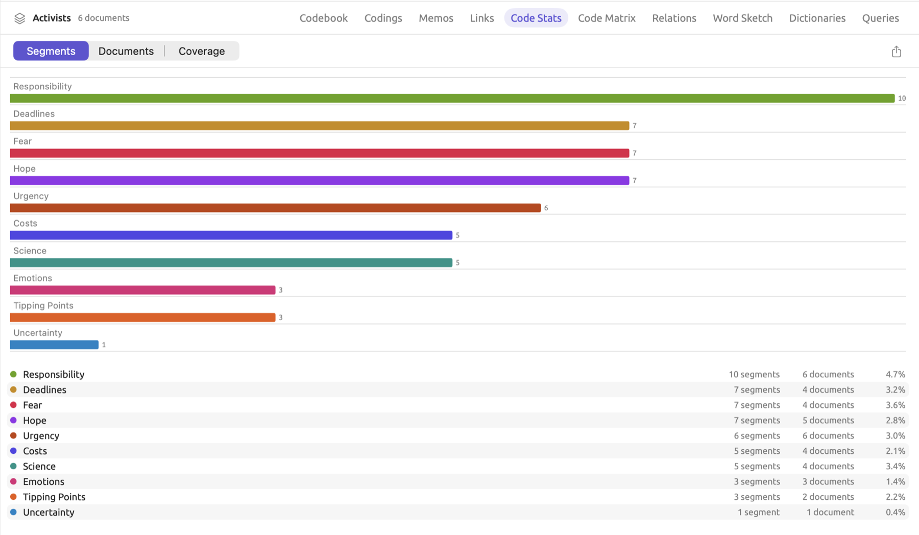
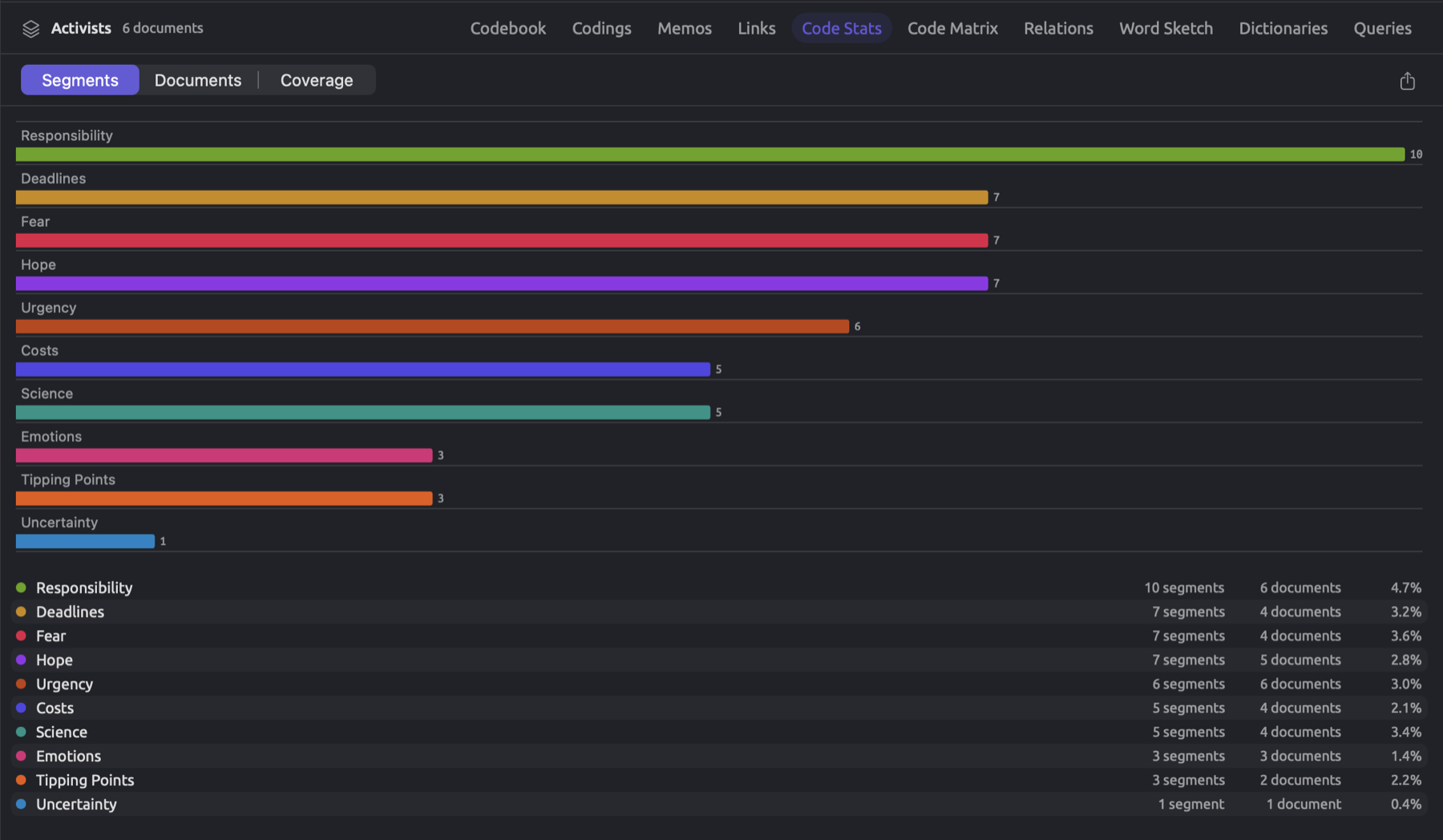
With the switch in the header (Segments, Documents, and Coverage), you can control which metric the bars show. Values are displayed at the end of the bars. Whatever the switch shows, the codes are always ordered from codes with many segments to codes with fewer segments. You can double-click a bar or row to read the segments of that code in the Codings view, or alternatively, right-click the row and select Show Codings from the shortcut menu.
- Segments is the total number of codings of the code in scope.
- Documents is the number of distinct documents in scope containing at least one coding of the code.
- Coverage is the proportion of characters spanned by the segments of the code relative to the total number of characters in scope.
For multiple documents, is the sum of characters covered by the code in each document, and is the number of characters in every document in the scope, coded or not. Using some rounded invented numbers, the six documents of the “Activists” set contain a total of 20,000 characters. Seven segments in the “Deadlines” code occur within four documents in total, covering 640 characters altogether. The table shows 7 segments and 4 documents, and coverage is calculated as:
Documents shows the distribution of codes among documents. While the “Responsibility” code has 10 segments distributed across all six documents, the seven segments of the “Deadlines” code distribute themselves among four documents. The coverage, then, will demonstrate if these segments consist of few characters or long passages of text. Since it represents a proportion of the whole scope, coverage decreases when the size of the scope increases. Since in the Code Stats of the whole project, the count also includes the characters from the documents of the skeptics and other texts, the coverage of a code seldom used by the skeptics, e.g., “Urgency”, decreases without changes in the segments.
Attribute Breakdowns below the table works exactly the same way as in the facet (see Attribute breakdowns above). Considering the supposed “Intensity” attribute, the breakdown chart of the “Fear” code in the “Activists” set displays its seven codings with 1 “Low”, 2 “Medium”, and 3 “High”, and 1 coding without a value.
The Code Matrix
The Code Matrix is essentially a table that lists every code of your scope as rows, and every document of the same scope as columns. Cells indicate the number of segments for each code inside each respective document. The last Total column provides totals per code for the whole scope, which match what Code Stats gives you. You use the Code Matrix in order to see what documents feature what themes, as well as to compare groups of documents by grouping their columns (see Grouping the columns below).
Codes appear ordered based on the ordering of your codebook, and subcodes are listed under their parent codes. If a parent code did not directly code a passage, such as “Speakers” in the project, then it too gets its own row above its subcodes despite having empty cells. Every document in your scope has its own dedicated column regardless of whether any coding was done within.
Cell colors tint according to which code they belong to and how many segments of that code they contain, the cell with the most segments taking the deepest tint of that code’s color. Empty cells represent zero. The Total column is framed instead of tinted.
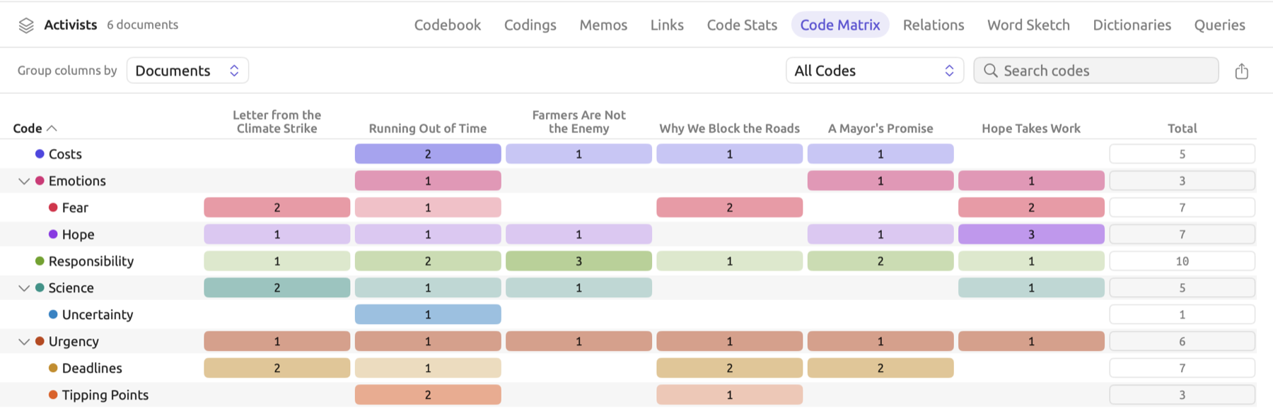
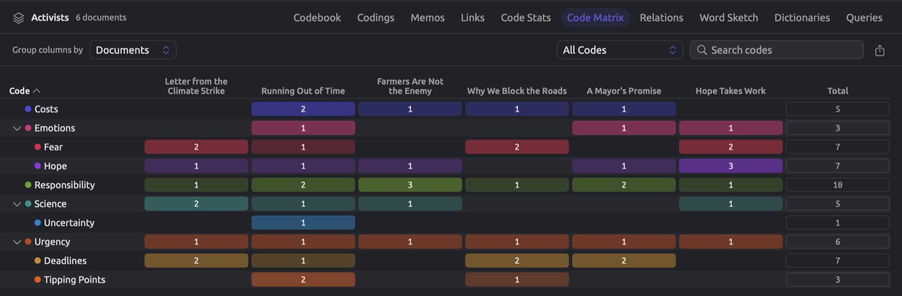
Here are three rows of the “Activists” set’s Code Matrix:
| Code | Letter from the Climate Strike | Running Out of Time | Farmers Are Not the Enemy | Why We Block the Roads | A Mayor’s Promise | Hope Takes Work | Total |
|---|---|---|---|---|---|---|---|
| Hope | 1 | 1 | 1 | 1 | 3 | 7 | |
| Responsibility | 1 | 2 | 3 | 1 | 2 | 1 | 10 |
| Deadlines | 2 | 1 | 2 | 2 | 7 |
Reading horizontally through a row will show you how a code is distributed among the documents. “Responsibility”, for instance, occurs in all of the documents, whereas “Hope Takes Work” holds three of the seven “Hope” segments. Reading vertically down a column tells you the themes relied upon within the document itself. First, look out for patterns in your data (codes absent from a group of documents, or conversely, codes mostly represented by a single document), then double-click a cell, or right-click it and choose Show Codings, to display its passages in the Codings view. Note that counts grow with document length and with how finely you segment, meaning that longer documents fill their respective columns more easily than shorter ones.
Above each matrix sits the header where the matrix tools reside:
- Group columns by enables grouping of documents together (more information under Grouping the columns).
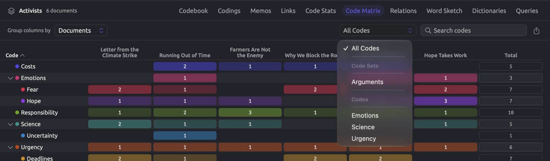
- The code menu (All Codes) limits the matrix rows to a code set (e.g., “Arguments” in “Climate Debate”) or a parent code and its subcodes.
- Search codes keeps the codes whose names contain what you type.
- Finally, the export button exports your table (please refer to Exporting tables and charts).
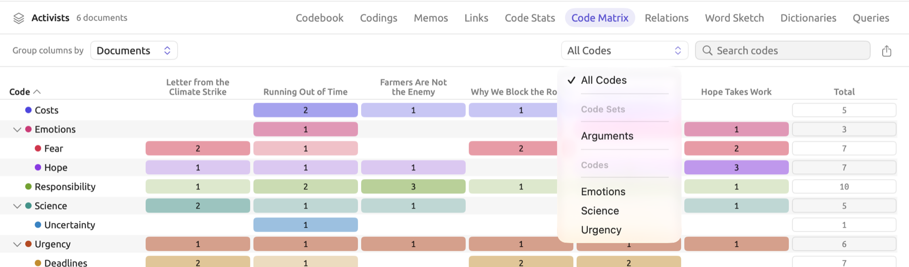
Clicking on a column heading sorts your rows according to that column, in descending order (the p column starts from the smallest p), whereas repeating it reverses the order. Document column headings sort your rows by most prevalent usage in that document. Clicking the Code column heading resorts the matrix rows back to codebook order. Only in that order does LemmaLoom indent your subcodes, enabling you to collapse a parent code with its adjacent arrow.
Grouping the columns
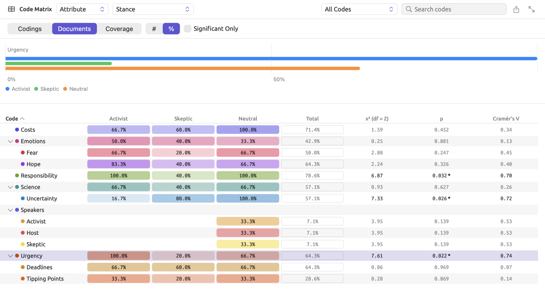
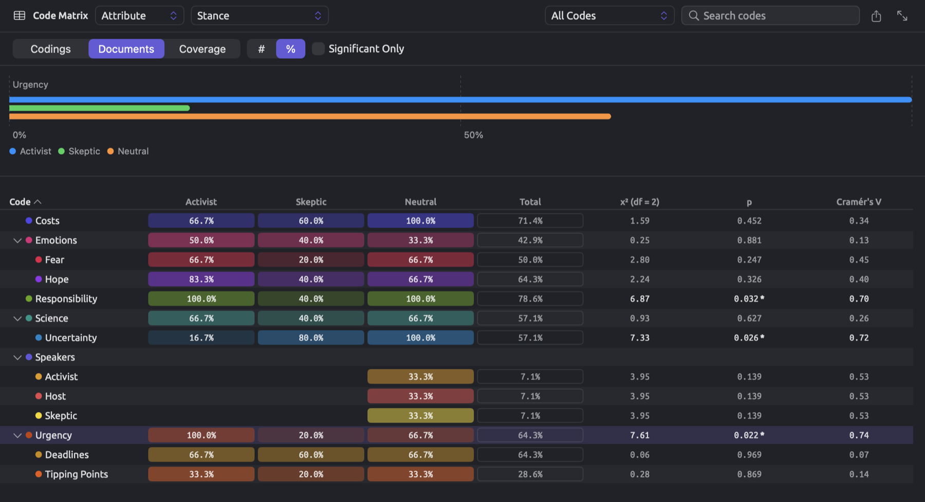
Group columns by rearranges the Code Matrix columns into groups of documents sharing a particular value. With it, you can compare kinds of documents, such as activists and skeptics, or print and online. “Climate Debate” assigns a “Stance” value to each of its originals. Therefore, you can group the documents by their stance and get a comparison between activist, skeptical, and neutral sources. The figure illustrates the project’s Code Matrix grouped by the “Stance” attribute with percentages of documents within cells.
To compare groups of documents:
- Open the Code Matrix of the project, a set, or a tag.
- In Group columns by, choose Attribute, Group, Language, or Format.
- For Attribute, choose the attribute, such as “Stance”, in the menu that appears beside it.
- In the row that appears below the header, choose what the cells count, and whether they show counts (#) or percentages (%).
The view now contains two panes, separated by a dividing line. At the top lies a bar graph showing the code you select in the table pane below, with separate bars, one for every group, each in a different color, with a legend underneath. Moving the dividing line provides additional space for either pane.
For column grouping options, Group columns by gives you:
| Choice | Columns |
|---|---|
| Documents | One column per document, which is the ungrouped matrix |
| Attribute | One column per value of the document attribute you choose in the second menu. Offered when the project has attributes. |
| Group | One column per document group, such as “Print” and “Online”, and Ungrouped for the documents in no group |
| Language | One column per language |
| Format | One column per kind of document (Text, PDF, Web Pages, Audio, or Video), as far as the scope holds them |
Documents with no value will appear in their own column called No value. Since all originals in “Climate Debate” have a “Stance”, grouping by “Stance” results in three columns; “Activist” contains six texts by the activists, “Skeptic” five texts by skeptics, and “Neutral” consists of the remaining three texts (“Heat Wave Report 2024”, “Carbon Tax Debate”, and “Radio Debate”). When documents are grouped by Group, the two ungrouped documents, “Heat Wave Report 2024” and “Carbon Tax Debate”, appear in their own column called Ungrouped. Each document belongs to only one column.
Columns appear in the order of their values. For pickers, this means the order of the choices; for numbers and dates, ascending order. For text and languages, alphabetical order applies. Order among document groups follows their order in the navigation sidebar. Columns No value and Ungrouped are always listed last. If there is a group, language, or format with documents in the scope, it will be shown in a column.
When dealing with numeric and date attributes, you will find yourself with an additional menu next to your attribute name. Reading Ranges or Values for numbers and Years or Months for dates, it controls how your attribute values are split into columns:
| Attribute type | Third menu | Columns |
|---|---|---|
| Integer, Decimal | Ranges (the first choice) | Up to four ranges, each holding about a quarter of the documents with a value |
| Values | One column per value | |
| Date | Years (the first choice) | One column per year |
| Months | One column per month, such as September 2024 | |
| Text, Picker, Boolean | (none) | One column per value; Yes and No for a Boolean |
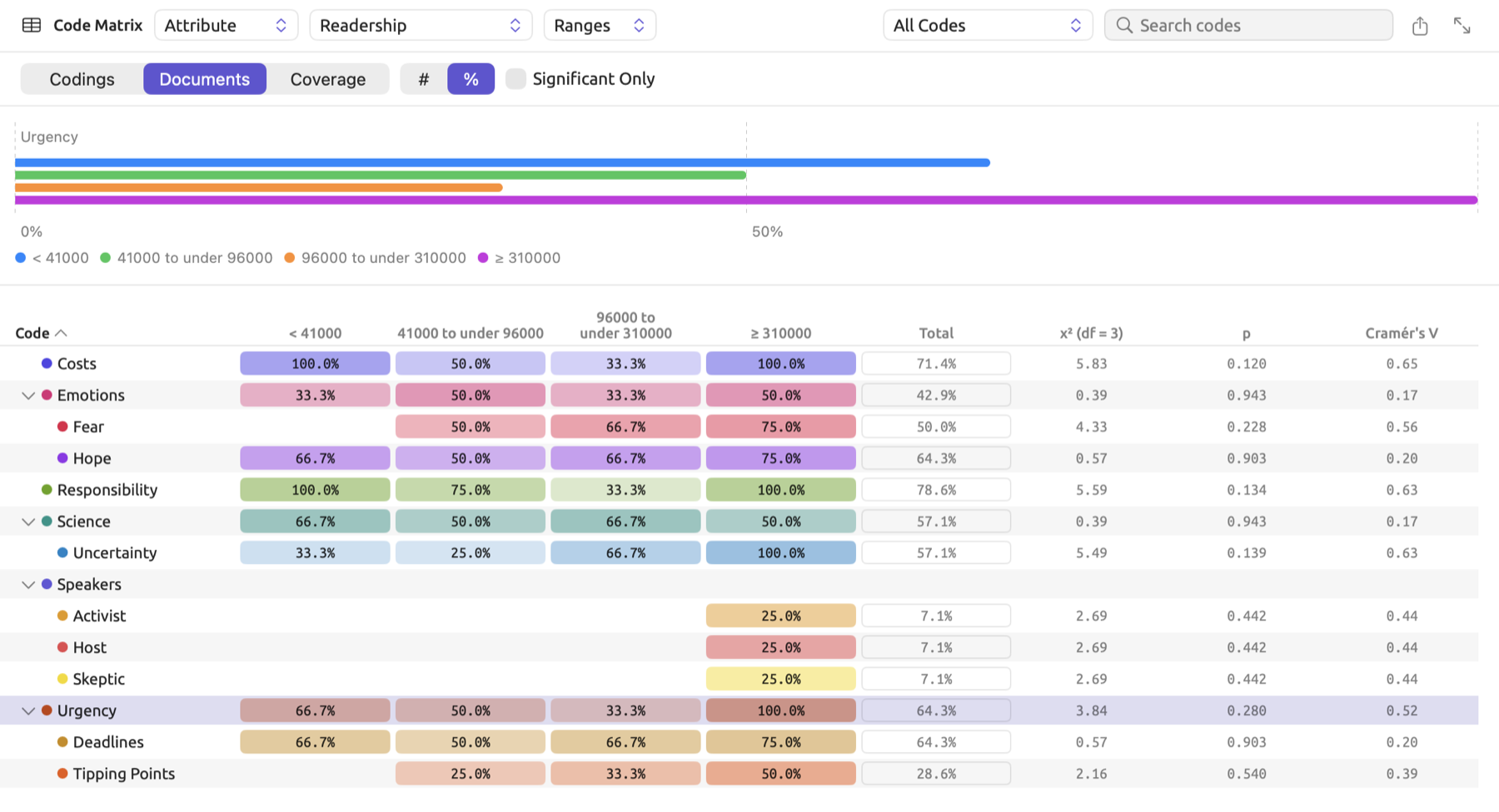
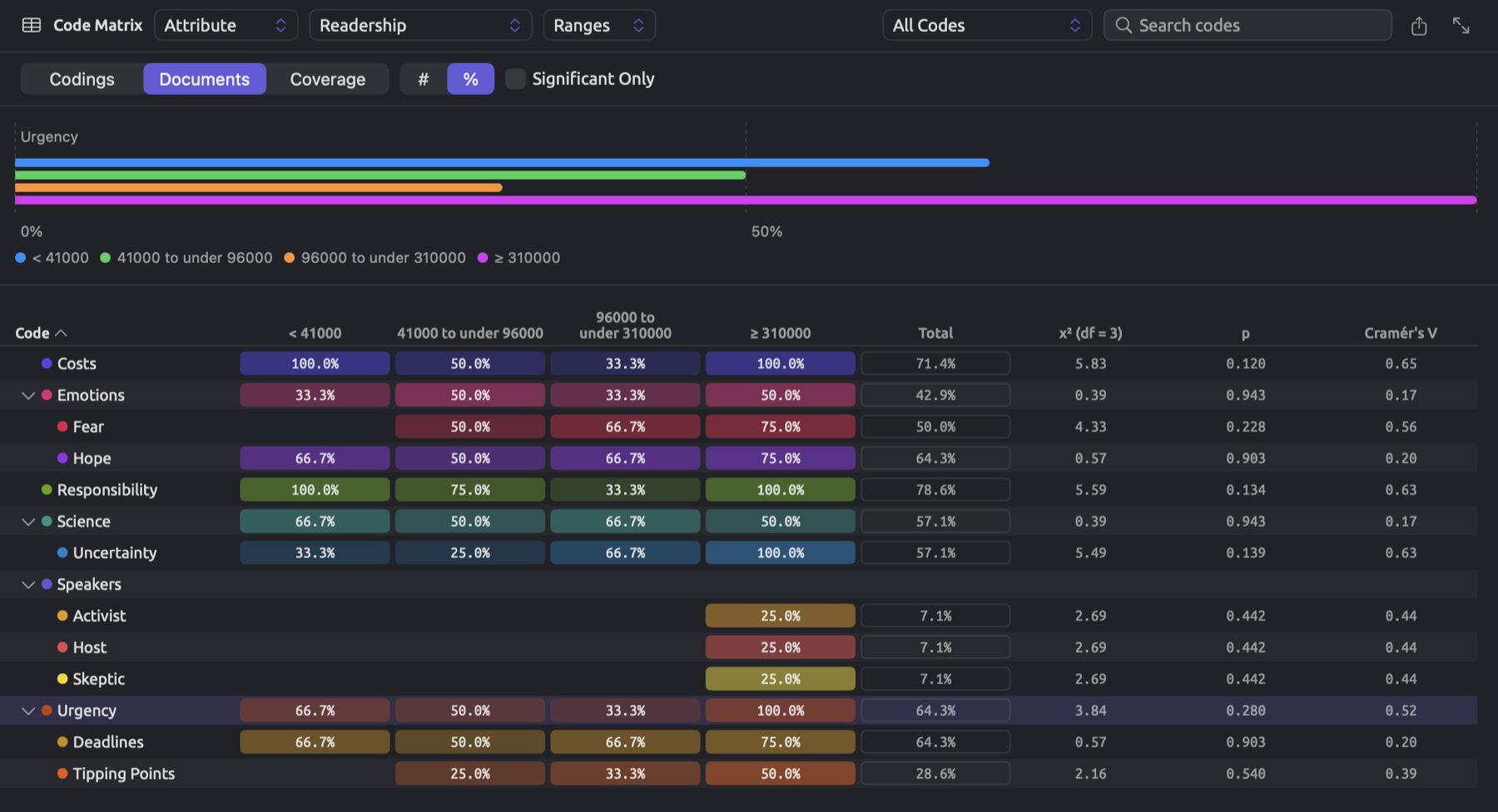
Ranges are calculated from values within a scope. Values are sorted from lowest to highest in LemmaLoom; their count is then multiplied by one quarter, one half, and three quarters; if necessary, any decimals resulting from multiplication are rounded down; finally, the value after that many values becomes a boundary. In the case of the fourteen originals within “Climate Debate”, the values for “Readership” are 3,100, 8,500, 23,000, 41,000, 57,000, 68,000, 72,000, 96,000, 186,000, 254,000, 310,000, 398,000, 412,000, and 875,000. Since , , and , the boundaries become the 4th, 8th, and 11th values, 41,000, 96,000, and 310,000 respectively. Thus, the range columns consist of < 41000, 41000 to under 96000, 96000 to under 310000, and ≥ 310000; there are 3, 4, 3, and 4 documents per range, respectively. A range encompasses its lower boundary and excludes its upper boundary. This means that a document such as “The Models Keep Missing”, which has “Readership” equal to 96,000, belongs to 96000 to under 310000. If several documents have the same value, fewer than four ranges may occur.
Counts and percentages
There will always be a second row directly underneath the header when grouping is enabled on the matrix, holding two switches and Significant Only. The first switch lets you define which type of count each cell will show. With the second, you could decide to show the count (#) or percentage (%) for each cell. The percentage value will divide the cell count by the group’s base number. Hover the mouse pointer over a group’s heading to see its base, such as Documents 6 for “Activist”.
| First switch | A cell with # | Base | A cell with % |
|---|---|---|---|
| Codings | The code’s segments in the group’s documents | All segments in the group’s documents, of every code | The share of the group’s codings that belong to the code |
| Documents | The group’s documents with at least one segment of the code | The documents in the group | The share of the group’s documents in which the code occurs |
| Coverage | The characters the code’s segments cover in the group’s documents | The characters in the group’s documents | The share of the group’s text that the code covers |
When you have documents of varying group sizes (in this case, six activist documents, five skeptic documents, and three neutral documents), you should consider choosing %. Typically, the best place to begin with the Code Matrix is Documents with %, because that indicates what proportion of the group’s documents contain the theme being analyzed.
The cells for each code row are shaded darkest for the group with the highest number for that code. The Total column represents the same values for the whole scope, including the documents under No value. Next follow the columns of the test (see Testing the differences between groups below).
Grouped by “Stance”, with Documents and %, the row for “Urgency” reads:
| Code | Activist | Skeptic | Neutral | Total | χ² (df = 2) | p | Cramér’s V |
|---|---|---|---|---|---|---|---|
| Urgency | 100.0% | 20.0% | 66.7% | 64.3% | 7.61 | 0.022 * | 0.74 |
All six activist texts contain the code “Urgency”. One out of five skeptics’ texts also contains the code “Urgency” (), as do two of three neutral texts (). In total, that’s 9 out of 14 texts, or 64.3 percent.
Testing the differences between groups
When there are two or more groups having a value among your columns, your table ends with a test for each code indicating whether there is an unequal presence of that code across the different groups beyond what could be due to random variance. Clicking on the heading of the p-value allows you to sort the codes based on p-value order from smallest to largest, while selecting Significant Only allows you to filter out any codes with p of 0.05 or above. Significant Only is disabled when fewer than two groups are available to be tested, showing Needs two or more groups when you hover the mouse pointer over it.
- As far as significance testing is concerned, the test always counts documents, regardless of switch settings. Within-document codings, however, are not independently observed, given a tendency by authors to repeat references to topics. Documents themselves can be considered independently observed data points.
- The tests exclude documents belonging to either the Ungrouped or No value columns. These do count in the Total column.
- If a particular test considers a code that exists in all tested documents, or none at all, it cannot possibly vary across any of the groups. Therefore, dashes replace the values in the test columns of that row.
- For two groups, LemmaLoom performs Fisher’s exact test, returning the columns p (Fisher) and Cramér’s V. If there are three or more groups, it performs the chi-square test, giving χ² (df = …) with the degrees of freedom, p, and Cramér’s V.
- Finally, when a code returns a p-value below 0.05, its test values are printed in darkened font along with a * immediately after its p-value. A p-value below 0.001 displays as < 0.001.
Fisher’s exact test for two groups
Organizing the document grouping of “Climate Debate” according to an attribute named “Stance” results in three groups. Reorganizing the column grouping according to Group gives rise to only two groups, “Print” and “Online”, both having six documents each. The two Ungrouped documents stay out of the test, leaving 12 in total. Eight of them contain the code “Deadlines”:
| With Deadlines | Without | Total | |
|---|---|---|---|
| 2 | 4 | 6 | |
| Online | 6 | 0 | 6 |
| Total | 8 | 4 | 12 |
In Fisher’s exact test, the totals are considered fixed, and the test asks how the eight “Deadlines” documents might have been shared out if the group made no difference. Imagine shuffling 12 playing cards, one per document, 8 of which were colored red, then dealing 6 of the shuffled deck randomly into “Print”; Fisher’s exact test calculates how many of all possible deals give “Print” each number of red cards.
The number of possibilities to pick items from , ignoring their ordering, is denoted and is referred to as “n choose r”. It is defined mathematically by the formula:
The notation represents the factorial operator, which multiplies together all integers greater than zero until reaching n; therefore . Choosing 2 items out of 4 would result in possibilities. More discussion on this counting process can be found in The one-sided Fisher’s exact test in Chapter 12, Word Sketch.
There are ways to distribute 6 out of the total 12 documents in a random deal. Dealing a hand of cards containing red cards entails choosing cards from 8 red cards and from 4 non-red cards; hence ways. A hand with 2 red cards has possibilities.
| Red cards dealt to Print | Hands | Share of all hands |
|---|---|---|
| 2 | 28 × 1 = 28 | 0.030 |
| 3 | 56 × 4 = 224 | 0.242 |
| 4 | 70 × 6 = 420 | 0.455 |
| 5 | 56 × 4 = 224 | 0.242 |
| 6 | 28 × 1 = 28 | 0.030 |
Fewer than 2 is impossible as “Online” contains only 6 documents, so at least 2 of the 8 red cards must be allocated to “Print”. Without the grouping having an effect on the allocations, “Print” should generally receive 4 red cards since 6/12 × 8 = 4.
The observed allocation yields “Print” 2 red cards. The test is two-sided, so it looks at both tails, summing the probabilities of all hands no more likely than the observed one. As a consequence, the test considers both hands receiving 2 red cards (28 possibilities) and hands receiving 6 red cards (28 possibilities), where “Print” receives 6 red cards such that every print document contains “Deadlines” and only 2 online documents do:
The “Deadlines” row has a value of 0.061 in the p (Fisher) column. An allocation with such an imbalance or greater happens around 6 times per 100 trials while randomly assigning 8 red cards. This value exceeds 0.05, hence the numbers in this row will not be printed darker and there won’t be a * for this row. There might actually be something to the difference here, but the test can’t discern that from luck.
The test is an exact probability calculation because it considers all possibilities for the allocation. The chi-square statistic of the same contingency table calculated using the formula for co-occurrences discussed previously returns a value of with . The problem here, however, is that all four expected frequencies (4, 2, 4, and 2) are lower than about 5, which makes it hard to rely on a chi-square distribution approximation. Therefore, LemmaLoom will report Fisher’s p for two groups.
The chi-square test for three or more groups
For three or more groups, LemmaLoom performs a chi-square test using the exact same table type, with a row per group containing the count of documents with and without the code. The “Urgency” row in the “Stance” example earlier relied upon this table:
| Stance | With Urgency | Without | Total |
|---|---|---|---|
| Activist | 6 | 0 | 6 |
| Skeptic | 1 | 4 | 5 |
| Neutral | 2 | 1 | 3 |
| Total | 9 | 5 | 14 |
Nine out of fourteen documents have “Urgency”. The expected counts can be found via ; here, equals fourteen, which represents the total number of documents. The expected counts in the row labeled “Activist” equal for documents with “Urgency” and for documents without “Urgency”. In the row labeled “Skeptic”, they equal and , respectively. For “Neutral”, they equal and . For “Activist”, . Other rows produce 4.27 and 0.01, so that:
An × contingency table has degrees of freedom. In the current case, ; you can locate degrees of freedom in the matrix’s heading, χ² (df = 2). With two degrees of freedom, the probability is 5 out of 100 of getting a equal to or larger than 5.99. The spreadsheet formula =CHISQ.DIST.RT(7.61,2) produces a . The row “Urgency” displays a 7.61 value, 0.022 with a *, and a Cramér’s V of 0.74, all printed darker.
Typically, it takes expected counts of five or so to use the chi-square distribution as an approximation to conduct hypothesis testing. In cases involving contingency tables this small, the p-value becomes a rather vague guide at best. By double-clicking the “Urgency” cell for “Skeptic”, you will begin reviewing “Net Zero Will Cost You”, the one skeptic text that contains “Urgency”, in the Codings view.
Cramér’s V
A p-value is influenced both by the number of documents and the size of differences between the proportions of codes. Effect sizes are measures of the magnitude of the differences themselves. Cramér’s V is a specific effect size that varies between 0 and 1, with 0 when the difference is null and a value of 1 being obtained in the extreme case where each group has the code in either all or none of its documents. The equation for V looks like this:
Here, is the number of documents tested, and is the smaller of the numbers of rows and columns in the table (two columns are used for presence/absence of the code, so , and thus V equals φ for two groups). So, for “Urgency”, ; while for “Deadlines” by Group, the chi-square statistic is 6.00 and therefore . This chi-square statistic was used solely for calculating the effect size; the actual p-value used was that of Fisher’s exact test.
Relations
The Relations view displays how much codes overlap each other within the scope’s documents. It can be used for exploring themes that writers bring up together, and it could even reveal whether two of your codes overlap too much, possibly describing the same concept.
The switch at the left of the header allows choosing between Grid, which displays codes vs. codes in tabular form, and Pairs, which lists the overlapping code pairs. In either case, φ and p values are calculated as for one document (see Co-occurrences in a document above). In this case, however, the four frequency counts are calculated across all the characters of the scope’s documents.
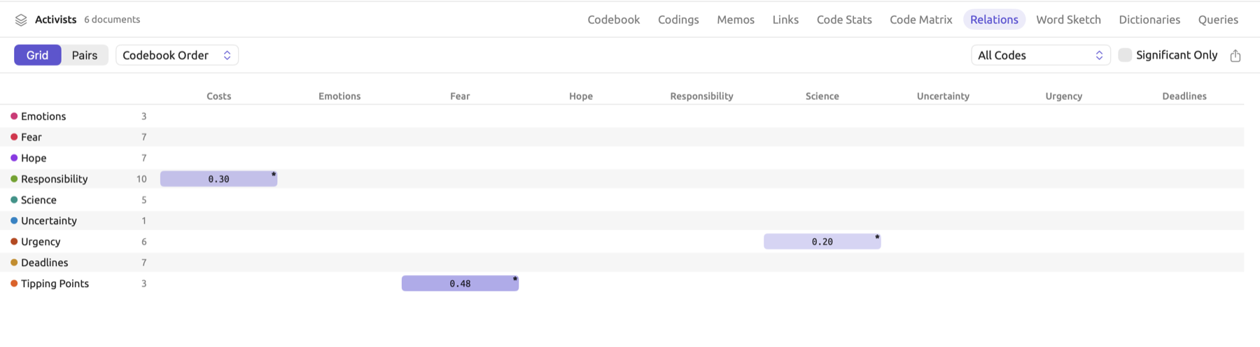
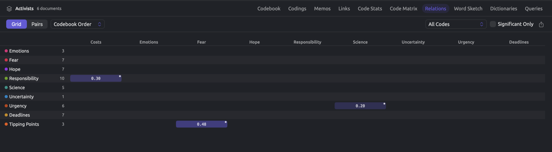
Grid is composed of rows and columns of codes. Each cell corresponds to a single pair, occupying a space along the lower left half of Grid. The content of a cell is φ rounded to two decimal places. Should the cell have p < 0.05, the cell corner gets a *. Cells are colored in the accent color based on the intensity of φ, with the most intense shading assigned to the greatest φ in Grid; an empty cell corresponds to zero overlaps between a pair of codes in the current scope. Next to each code name on the left side is the number of segments the code has, and hovering the mouse pointer over a cell reveals the number of overlaps and p-value. Codes are ordered according to the selected sort criterion, which is done via the sort menu adjacent to the switch. Sorting codes by Codebook Order preserves the order of appearance in your codebook, while sorting codes by Clustered places strongly overlapping codes adjacent to each other in Grid.
Unlike Grid, Pairs shows one pairing of two codes per row, and includes five columns (Code A, Code B, Overlaps, φ, and p). The table starts with the largest φ; if necessary, you can always re-sort by clicking the respective column headers. Should you wish to retain any pairings whose code names contain certain substrings, use the Search codes field. Each cell within Overlaps represents the count of overlaps, with two segments that overlap within the same document counting as one overlap. Essentially, it is CO-OCCURS WITH in the Codebook view (see The Codebook view in Chapter 7, Coding).


Both Grid and Pairs provide a filtering function based on a code set or on a parent code and its subcodes from the code menu (All Codes). Both tools allow for narrowing overlaps shown to the significant pairings only (Significant Only), with p values less than 0.05 being considered significant.
The “Activists” set reveals three pairs of overlapping codes, “Tipping Points” with 3 segments and “Fear” having 7 segments, overlapping 2 times; “Costs” and “Responsibility” overlapping just as often but having 5 and 10 segments, and “Science” with “Urgency” overlapping once. Naturally, more segments equate to more possibilities of overlapping, so always cross-check overlaps against the numbers of segments, or look at φ values. The latter takes into account the number of overlapping characters relative to each code’s size.
Finding * is easier when you are analyzing an aggregated table rather than an individual document, because it accounts for all characters contained in every document within the current scope. Trust the φ values, but bear in mind that the significance may arise purely because of overlap in one large document alone. To examine the overlapping segments, you could double-click cells in Grid or rows in Pairs, or use the Show Codings command from the shortcut menu. In response, Codings will display the overlapping segments of the code preceding the other code in the codebook (i.e., Code A in Pairs), along with both code names in the header like Fear · Tipping Points.
Exporting tables and charts
All tables and charts throughout this chapter include an export button located in their heading or view header area. This is represented as a square icon with an upward pointing arrow. When only the CSV export format is available, such as in Co-occurrences, the Codeline, the Codings view, and Pairs in Relations, pressing the export button opens the save dialog directly. Otherwise, pressing the export button produces a menu offering PNG and PDF exports first, then CSV if the chart has a table behind it. For information on exporting the Codes, Codings, and Links facets and the Codebook, Memos, and Links views, refer to Chapter 7, Coding.
- Set up the view as you want it, with its grouping, switches, search, or filter.
- Click the export button, and choose a format if a menu opens.
- The save dialog suggests a name made of the document, set, or project and the kind of table, such as
Running Out of Time-co-occurrences. Choose a folder, and click Save.
Your file data reflects what the view shows. When searching and filtering in Codings, the results carry over to the file data, and so too do the code menu, Search codes, and Significant Only in the Code Matrix and Relations, and the choice of counts or percentages in the Code Matrix.
| Place | Formats | Columns of the CSV file | Suggested name |
|---|---|---|---|
| Code Stats facet, Code Frequencies & Coverage | PNG, PDF, CSV | Code, Segments, Characters, Coverage (%) | Running Out of Time-code-frequencies |
| Code Stats facet, Co-occurrences | CSV | Code, Code, Overlaps, Characters, φ, p | Running Out of Time-co-occurrences |
| Attribute Breakdowns, each chart | PNG, PDF, CSV | Attribute, Value, Count | Running Out of Time-Fear-attributes |
| Portrait, Mosaic | PNG, PDF | Running Out of Time-mosaic | |
| Portrait, Codeline | CSV | Sentence, Codes, Text | Running Out of Time-codeline |
| Codings view | CSV | Document, Code, Text, Start, End, then one column per attribute | Activists-segments |
| Code Stats view | PNG, PDF, CSV | Code, Segments, Documents, Characters, Coverage (%) | Activists-code-statistics |
| Code Matrix | PNG, PDF, CSV | Code, then one column per document or group, and Total | Activists-code-matrix |
| Relations, Grid | PNG, PDF, CSV | Code, Segments, then one column per code | Activists-code-relations |
| Relations, Pairs | CSV | Code, Code, Overlaps, Characters, φ, p | Activists-code-pairs |
There is the option to export Co-occurrences and Pairs as CSV files too; for these files specifically, Overlaps refers to how many pairs of segments overlap, indicated as 1× in the facet, and Characters to how many characters two codes share. φ and p both have four decimals, hence very small values of p appear as 0.0000. In the case of Codeline CSV, Codes refers to the row’s codes, which are semicolon-separated. Empty cells in the Code Matrix CSV are filled with 0. The Grid CSV, however, keeps the view’s lower half, φ being rounded off to four decimals, and an empty cell wherever there was no overlap between two codes.
When a grouped Code Matrix is exported to a CSV file, a column is dedicated to every group, with (%) after its name if the percentage option was selected (%), followed by Total and the test (χ², df, and p, or just p (Fisher)). Finally comes Cramér's V. The first row in a grouped Code Matrix CSV will include the bases of each group and the label indicating their content (e.g., Documents). Percentages are written out in numeric format with two decimals (e.g., 66.67). Test results of p-values will be outputted with six decimals, while those of χ² and Cramér’s V will have four decimals. A code lacking a test will have empty cells in the test columns.
PNG and PDF exports for tables and charts are generated anew for the file you wish to export, using colors according to the active theme. The table within a grouped Code Matrix export image includes its bases, along with the test columns. To learn more about CSV exports and how pictures look in a dark theme, check Exporting tables and charts in Chapter 22, Exchanging and Exporting.