Query Results and Statistics
The Find, Pattern, and Where conditions determine what hits a query will collect, whereas the Show condition decides what you see of them. It could list out the hits, count them, run statistical tests comparing groups of documents, track hits through each document or across time periods, find their collocates and keywords, and/or determine co-occurrences among them. Each and every one of these results may be exported in tabular form, as a text file (including the query used to produce the result), or as an image. If you would like to know more specifics on these individual conditions, check out Chapter 15, Building a Query.
These examples use “Climate Debate”, which is the example project of this guide. In order to replicate the examples, choose File ▸ Import ▸ Example Project, and LemmaLoom will load the project in your preferred interface language. Most numeric figures in the examples are invented for simplicity’s sake; hence, they differ from those displayed in the screenshots. Where a particular example makes use of the example project’s own counts, such a fact will be noted explicitly.
Key terms
- A hit is one of the things returned from executing a query, whether it is a word, sentence, coding, speaker turn, document, or code. The bar above the results displays the total number of hits in a query’s output, for instance, 312 Hits.
- A Group By key groups hits by one of their features, such as codes, speakers, and attributes like “Stance” of their document. Each distinct value of the key becomes a separate row in the output.
- A measure refers to a quantitative value displayed in a row of results; measures may refer to the number of hits or documents, rates, coverage, or shares.
- A rate refers to dividing the number of hits by the number of words in which the hits occurred. With rates, comparison of texts of varying lengths is possible since normalization takes place.
- A document-level key refers to a type of Group By key which has only one value for each document. Examples of document-level keys are attributes such as “Stance”, the document’s group, its language, and the document itself. Tests under Compare rely on document-level keys to run since comparisons take place on documents.
- A test estimates how easily chance alone could produce the differences you observe between groups. It returns a p-value and an effect size, both explained in p-values and effect sizes later in this chapter.
Choosing what to show
Clicking on the Show condition will show you up to seven kinds of results depending on what your query is. However, not all seven will appear depending on what the query analyzes (i.e., the unit of analysis, what Find looks for) and what range it is searching through (scope, at document, set, or project level).
| Show | What you get | Offered for |
|---|---|---|
| List | The hits themselves, as a concordance or a table of records | Every query |
| Count | One number, or numbers for the values of one or two Group By keys | Every query |
| Compare | Numbers for each group, with a statistical test | Sets, projects, and All Projects |
| Over Time | A line chart, or a strip per document showing where the hits fall | Passages and Documents |
| Collocates | Words that occur near the hits more often than chance would suggest | Words, Pattern Matches, and Text Matches |
| Keywords | Words a set uses more or less often than a reference | Words, in a set or project |
| Network | A table of how often values occur together | Passages |
Passages are all the units of analysis that have a place in your document. This includes everything in the Find menu aside from items found in Library, such as Documents, Codes, and Sets.
It is common to begin with List. Going over the hits returned by List can tell you if you’re getting what you need from your queries. Once satisfied with the quality of your hits, using Count gives you the total number of hits as well as how many there are in relation to your codes, speakers, or attributes. Compare statistically assesses whether the difference observed between document groups is greater than what could happen by coincidence. If you are dealing with location and time questions, Over Time would be useful. Collocates and Keywords both solve problems related to vocabulary, while Network allows visualization of co-occurrences between your codes or other values.
Depending on the kind of result chosen, there are various options available in the Show condition. A Limit selected in List, Count, or Compare stays applied when switching to Collocates, Keywords, or Network. Although the Limit checkbox itself disappears from view, the limit still applies until you switch back, deselect it, and return to the chosen kind.
The results area
Your results show directly underneath the query builder wherever you create your queries. In sets and projects, your results occupy all the horizontal space of the Queries section beneath the left column and the conditions. In the Queries window (Window ▸ Queries), your results take the full horizontal width too. The divider bar between builder and results allows you to resize the two areas according to preference. If you are viewing a document, you will find the Query facet of the inspector has your results in its lower part.
If a query does not involve analyzing the texts of a large set, project, or All Projects, it is run automatically whenever you edit it. But queries analyzing such texts wait for you. You can recognize these kinds of queries by noticing that the Run Query button now appears in their results areas. See Running a query in Chapter 15, Building a Query for specifics regarding the set, project, or All Projects sizes where this happens. Running your queries is achieved via the Run Query button in the results area, the ⌘R keyboard shortcut (Edit ▸ Run Query), or the triangle icon in the bar above the builder.
Background-running queries occur asynchronously in order to enable you to keep reading or coding during their execution. Background-running queries have their own progress ring in the bar above the builder, which becomes active when the execution starts, indicating the completion rate in percentages of how many documents they have analyzed. As long as the execution is ongoing, you can find the Stop button replacing the triangle. Your results get updated in real-time as your query analyzes your documents, remaining faded till execution is done. The lists in the results only show at maximum the first 5,000 hits until the execution ends. Also included at the bottom of those lists is the number of total hits found, like Showing 5,000 of 12,431. Lists sorted in any order other than Document Order stay in document order until then and are sorted afterward. Clicking Stop ends the execution at any time and keeps the partial results. Keyword lists appear solely once queries are complete.
The bar at the top of the results area, or results bar, summarizes the results. It gives the hit count of most queries, e.g., 312 Hits. Library item queries show item counts, e.g., 14 Results, whereas networks report the number of values they link, e.g., 10 Nodes. Aside from these counts, the bar indicates how many documents were read when the query had to leave some out (see Documents left out below), and the value you have drilled into (see Drilling down later in this chapter). The right side of the bar includes the Filter field (for applying filters in query results), Export (the box with upwards pointing arrow), and Open results in a window (two outward-pointing arrows). Within a document’s Query facet, the bar holds only the summary, the number of documents read, and the drill-down value. Instead, Export lies in the bar located at the top of the facet above results.
If a query cannot run, the results area explains the reason, like Needs a set or project, No set chosen, or Invalid pattern. The triangle button is disabled in those cases. Its tooltip gives the same reason. If there were no matches returned after running the query, the results area displays No matches.
Documents left out
Queries finding Words, Pattern Matches, Sentences, Phrases, Noun Chunks, or Findings will only work on documents that have been indexed. Those documents that haven’t been indexed will be excluded, as will documents in languages other than English, German, and Chinese. Results using word counts, e.g., Per 10,000 Words, the rank test, or DP, leave out such documents as well. The results bar will inform you of how many documents have been read, e.g., 12 of 14. This figure also appears if you stop your query prematurely.
A rate, count, or statistical test performed on 12 out of 14 documents reveals nothing about those other two documents. For additional guidance on seeing and finishing the indexing of each document, please refer to Chapter 21, Analysis and Indexing.
Filtering the results
The Filter field narrows what the results show. Imagine you received hundreds of hits from one query, which include a few hits from just one document or from a particular code. You now wish to focus solely on these hits; the solution lies in typing a few characters in the Filter field. Only rows containing that text will remain visible to you, while capitals will be ignored.
How filters behave varies depending on which type of result you are working with. List filters assess the text of each hit and its surrounding context, the title of documents, and any extra columns such as code or speakers. Filters for counts, comparisons, collocates, keywords, and networks filter based on the name of the row. For Position in Document strips, filters evaluate document titles only. All result types besides a single number and a line chart can use filters.
Keep in mind that filters simply conceal rows. The overall count of hits reported above in the results bar, the figures in all rows, and any test still consider all hits made in total. Limit defines how many hits will actually appear in the list; thus, applying a filter affects only the hits left after the limit. Exports keep only the rows that pass the filter.
Results in a window
Pressing the Open results in a window button on the right side of the results bar opens the currently displayed result in a new window with its very own results bar, Filter field, and Export button. This window has a title with the name of the query, scope, and value that you’ve drilled into (if any), and this name is repeated with the number of hits found next to it.
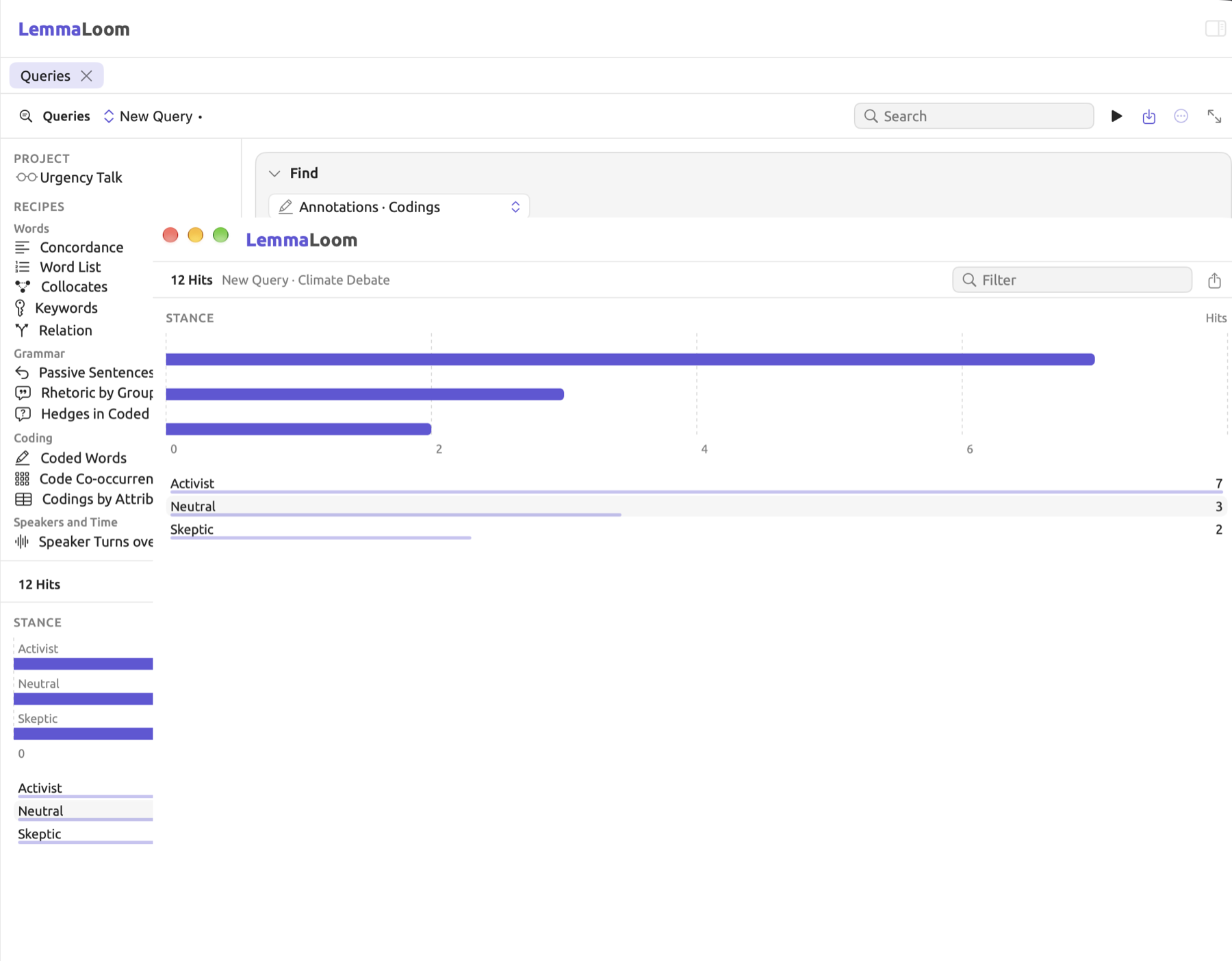
Since this window retains the state of the result from when you opened it, you may adjust the query or scope, run it again, and compare its results against the previous results side by side. This could mean setting “Fear” codings by stance against “Hope” codings by stance, among other possibilities. Drilling down and opening hits function within the window too.
Until the query finishes running, the button remains disabled. Clicking the window button in the bar above the builder opens the entire query in the Queries window (see The Queries window in Chapter 15, Building a Query).
Lists
List presents the hits actually retrieved by the query. Hits which occur in some part of the text appear in concordance format, whereas library objects such as documents or codes appear in table format. If you ever come across an unexpected count, consult List for clarification.
Concordance
Concordances are lists of hits on word(s) or passage(s) that show each occurrence of that word or passage in the middle column, with its context on either side. When scrolling down the middle column, you will notice multiple uses of a particular word or passage at once.
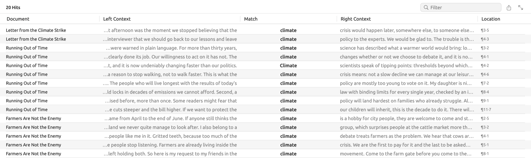
The concordance columns are as follows:
- Document represents the document that holds the hit inside of a set, project, or All Projects.
- Left Context and Right Context show up to 70 characters prior to and after the hit, replacing all line breaks with spaces.
- Match refers to the actual match found during the search process. If any match exceeds 400 characters, it gets cut down with “…”.
- There are also several other columns related to the query’s unit type. These are Code in regard to codings, Content and Linked Code in relation to memos, Comment related to bookmarks, Other Document and Relation pertaining to links, Speaker and Start regarding speaker turns, Finding associated with analyzer findings, Phrase Label and Phrase Function in regard to phrases, and Translation Text concerning alignments.
- Location provides exact information as to where within a document a particular hit occurs. Such locations resemble, say, ¶4·2, meaning the second sentence of the fourth paragraph of said document. If a hit takes place within a document that has not been indexed yet, the sentence numbers will be omitted, so that locations would instead resemble ¶4.
- Category displays in case you have categories involved or used Color By while creating the query. Likewise, Project displays should you choose the All Projects option. Finally, Score appears in case sorting happens by the hit score.
Each hit in the list can take you right to its place in the document. This may be accomplished by double-clicking the hit itself, selecting the hit and pressing the Return key, or selecting the hit and picking the Go to Source item from its shortcut menu. LemmaLoom switches over to displaying the document containing the hit in the preview tab (unless it is open already) and highlights the match. In case your hit belongs to another project, LemmaLoom switches to that project.
Within a document’s Query facet, hits get presented as a narrower kind of concordance view. Every hit occupies its own row and displays both preceding and following words as well as a match in bold between them, with the location beneath. Whenever hits appear one after another in the same location, the location is displayed once, for the first hit only. A click on the hit makes it show up in the reader.
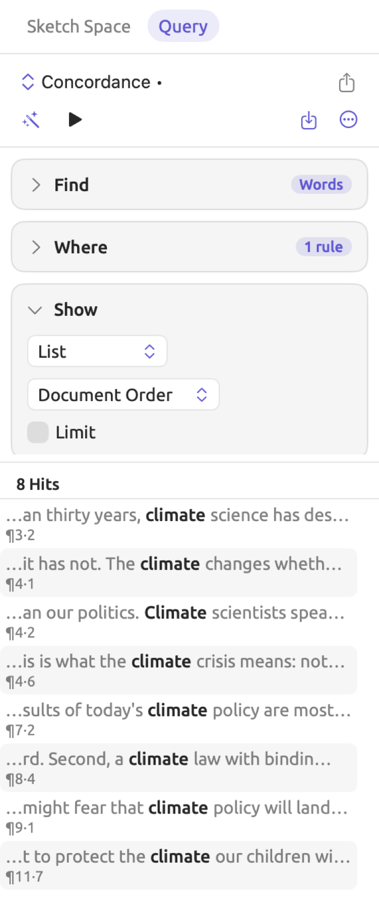
Sorting hits within lists occurs based on the menu showing Document Order in the Show condition. The choices are:
- Document Order keeps the order of the set or project, and of the text. This is the default.
- Match sorting occurs alphabetically according to matches themselves.
- Left Context sorts hits by the preceding words, reading left contexts backwards starting from a match position.
- Right Context sorts hits by subsequent words occurring within the right context.
- Document sorts hits alphabetically by document titles.
- Frequency sorts by hit frequencies, counting appearances of hits’ matches. Ignored in frequency counts are all differences caused by capital letters and accents. The hits that repeat most often come first.
- Score orders hits according to their scores, placing hits that scored better on top. Only if queries feature a weighted word list created with Passages Like a Code or Freeze Values would this option be available. Also, in this sort mode, hits that contain fewer than two words from the list get ignored. Thus, the total number of hits drops in comparison with the initial number. See How sentences are scored in Chapter 17, Query Patterns and Discovery and Freeze Values in Chapter 18, Using Query Results for more.
There are restrictions regarding the maximum number of hits a list shows. They come in the form of two settings. Select Limit from the Show condition and set the desired hit number; it starts at 50 and goes up to 10,000. Another restriction caps every list and appears in the Options condition as Limit, starting at 5,000 and allowing values between 1,000 and 200,000 in increments of 1,000. Every time you have queries returning more hits than those numbers allow, a line appears under the list, for example Showing 5,000 of 12,431. Note that the hit count in the results bar always includes every hit. When sorted by Document Order, the list keeps the first hits found. Otherwise, LemmaLoom analyzes all of the hits returned by queries to sort them in your specified manner, retaining only the top of the sorted list. It is advisable to keep your lists short. Set high hit limits only when you need every hit, such as for a complete export.
Records
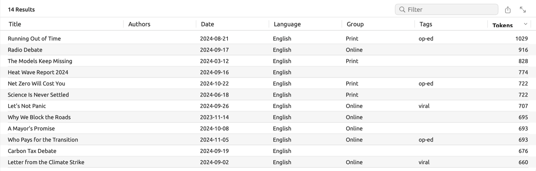
When Find is set to one of the Library units, List produces a tabular view with each row representing an item in your project. Use List when wanting to survey the documents, codes, and/or other items in a project with respect to their properties next to each other. For example, List can be used for finding documents lacking dates or rarely-used codes. The first column is titled Title for documents, and Name for everything else. The other columns depend on the unit.
| Find | Columns after the name |
|---|---|
| Documents | Authors, Date, Language, Group, Tags, Tokens |
| Codes | Path, Codings, Coded Documents, Tags |
| Code Sets | Codes |
| Sets | Kind, Documents |
| Groups | Documents |
| Attributes | Type, Owner, Values Set |
| Tags | Uses, Projects, Documents, Codes |
| Dictionary Terms | Category, Dictionary, Hits |
| Analyzers | Languages, Legend Keys |
| Projects | Tags, Documents |
Click a column header to sort by that column; clicking it again reverses the order. Numeric values will sort based on number size while text will be sorted in alphabetical order. You may configure the starting order with the menu showing Document Order in the Show condition to be Name or Document Order. To view a document, double-click its row, select the row and press Return, or right-click it and choose Go to Source.
Counting
Count transforms hits into numbers. In its most basic form, with no Group By key, Count returns a single number, while adding one or two keys yields lists and tables respectively. A count represents the documents exactly as they stand. If you wish to ask whether the difference between groups exceeds the level of chance, use Compare (see Comparing groups later in this chapter).
Counting all hits
If Group By is left blank, Count returns one big number with the name of the measure below it (the default being Hits, unless you’ve changed the menu showing Hits), along with a line saying something like 7 hits in 4 documents. With regard to the “Climate Debate” project, the code “Fear”, which belongs under “Emotions”, is applied to any passage expressing or invoking fear. Counting its codings in the “Activists” set shows how often the activist texts used fear, and in how many of them.
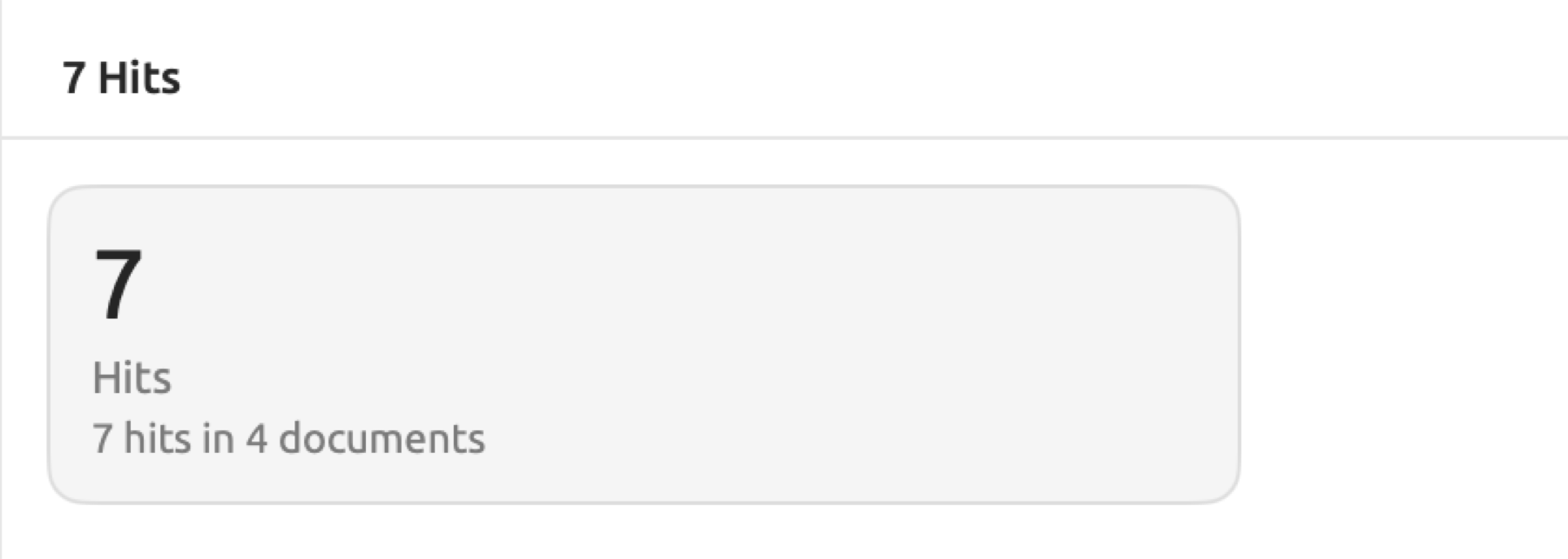
Counting the codings of one code entails:
- Open the Queries section of the set or project.
- In Find, choose Codings.
- In the Where condition, click Add and choose Add Rule.
- In the new rule’s field menu, choose Code.
- Choose the code as the rule’s value.
- In Show, choose Count.
The counting process follows similar procedures regardless of what a query retrieves. When using Words in Find and a rule on Lemma, for instance, it counts the number of occurrences of a word.
Counting by group
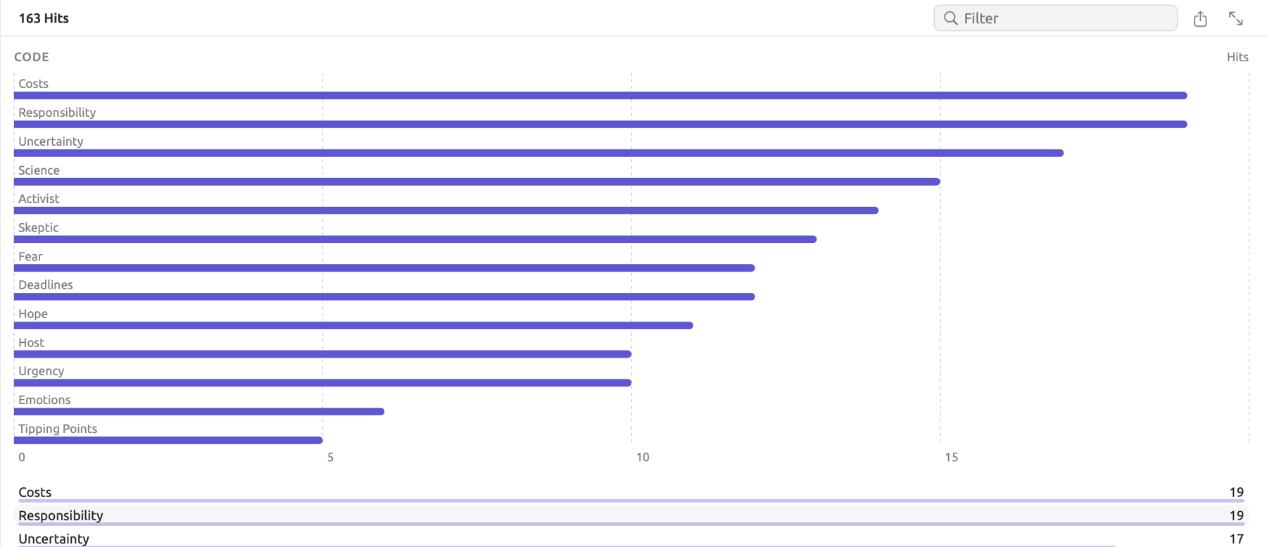
The Group By key illustrates the distribution of the hits. In the “Climate Debate” example, each document carries a “Stance” attribute (i.e., “Activist”, “Skeptic”, or “Neutral”). So, grouping the codings in the project by code, and then by “Stance”, shows which codes each side uses in the debate, as shown in the figure.
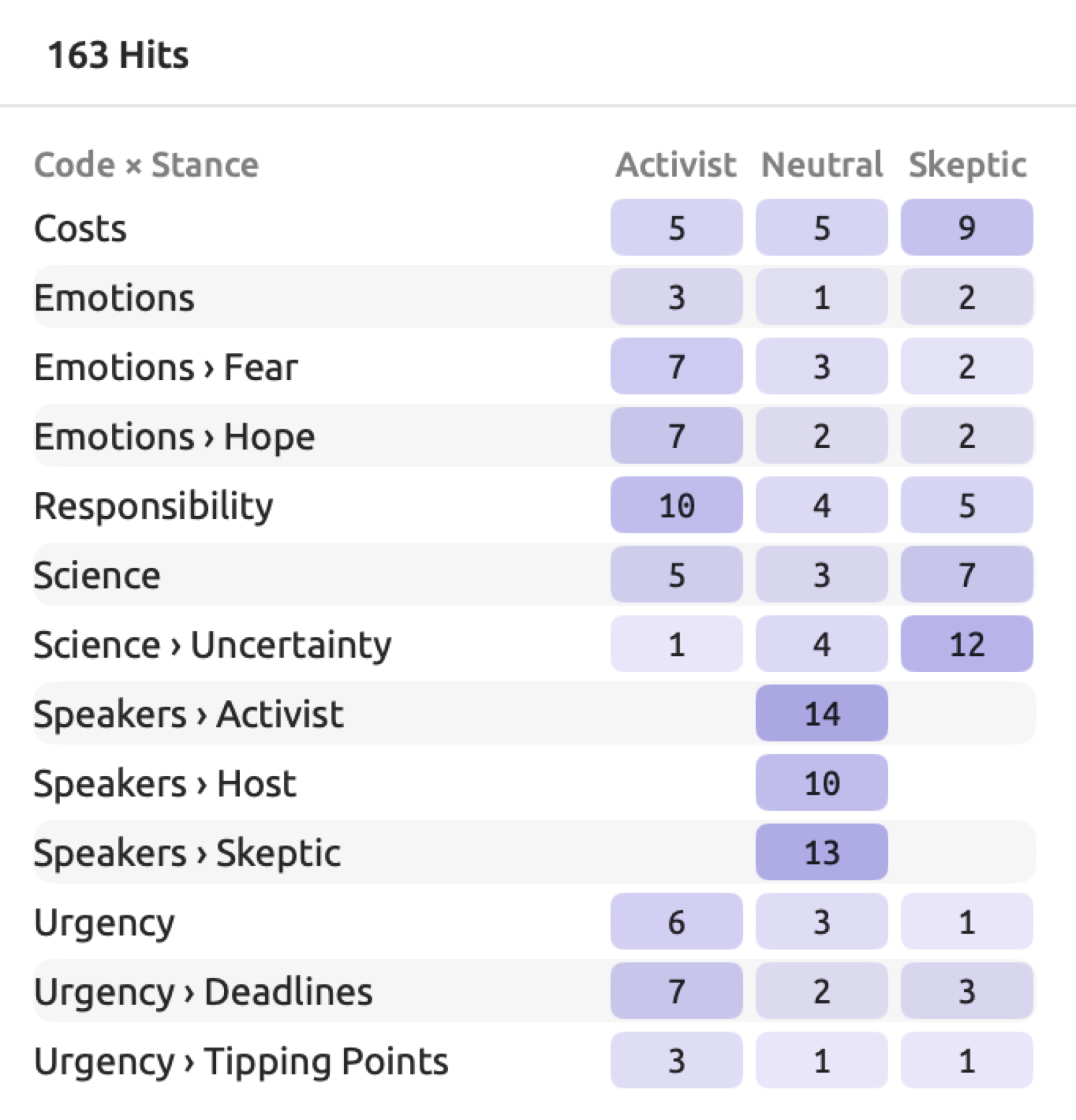
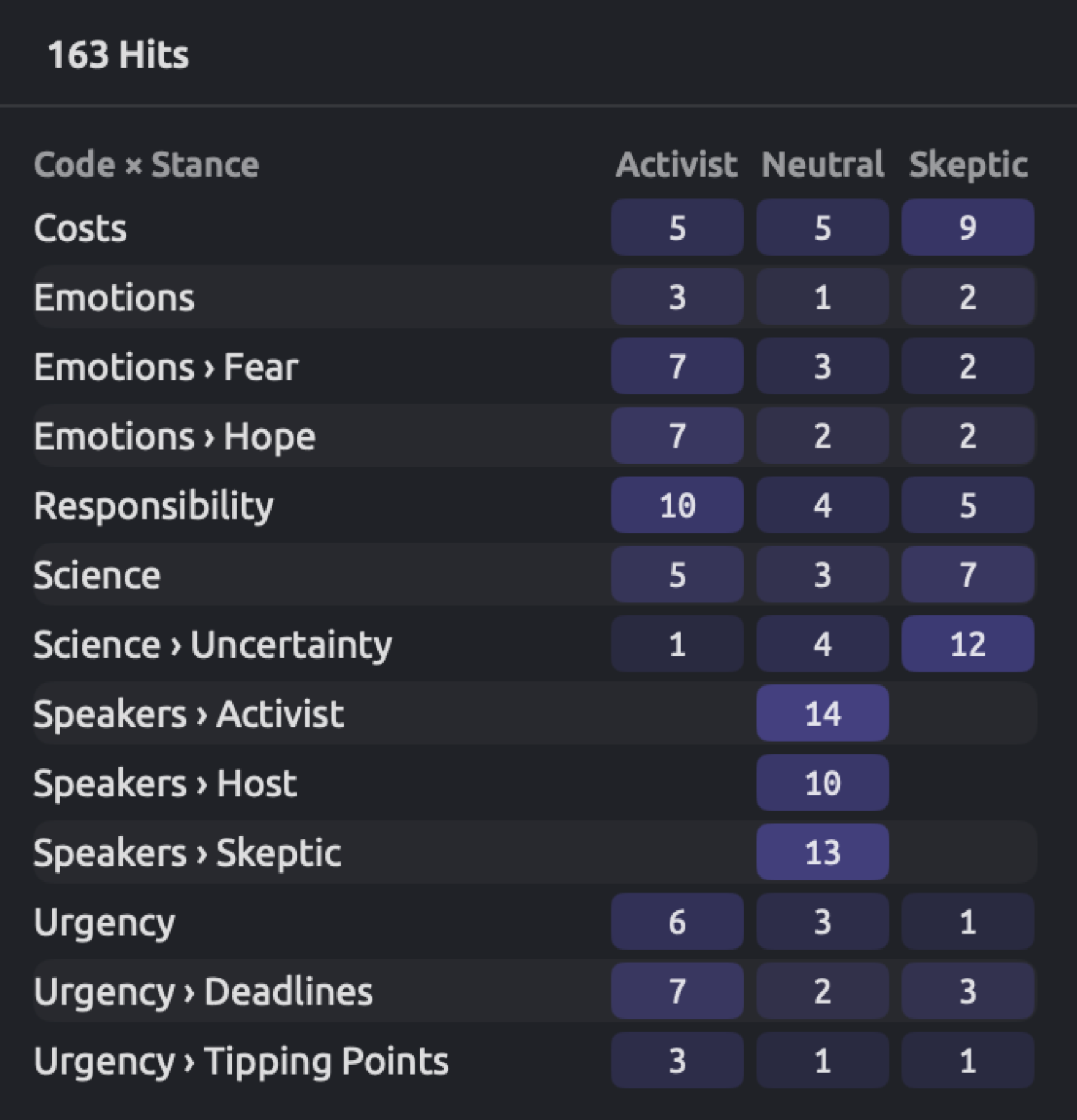
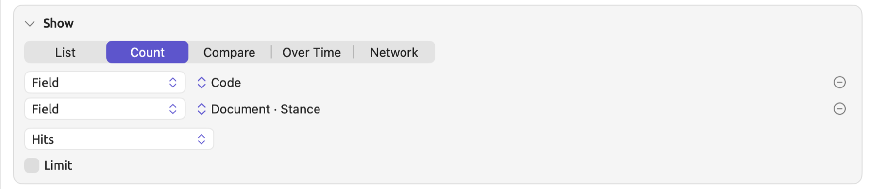
For counting hits by group:
- In Show, choose Count.
- Click Group By. A key row appears, with the menu showing Field.
- In the field menu beside it, choose the property to group by, such as Code.
- For a table, click Group By again.
- In the second row’s field menu, choose the second property, such as Attribute ▸ Stance.
With one key, you get a list with a single row per value sorted largest to smallest. Each row gets a narrow bar showing its value relative to the largest value. If your list ends up having between 2 and 30 rows, a bar graph is placed above the list, except in the inspector. List rows that represent categories have colors assigned to them.
Two keys result in a list becoming a table. Rows correspond to the values of the first key and columns to those of the second key. The corner names both keys, as in Code × Stance. Cell values represent measures corresponding to both keys at the same time, with greater values being colored in progressively darker shades. Cells without hits stay blank. Hovering the mouse pointer over any given cell lets you inspect the respective row and column labels. You may use tables to explore two properties at once, such as whether skeptics use different codes than activists. The Codings by Attribute recipe, under Recipes in the left column of a Queries section, builds a similar table, by code and by group.
Group By keys
The menu showing Field in each key row has these options for sources:
| Group By | Groups hits by | Offered for |
|---|---|---|
| Field | The value of a field chosen in the field menu | Every query |
| Document | The document | Passages and Documents, in a set, project, or All Projects |
| Project | The project | All Projects |
| Language | The document’s language | Passages and Documents, in a set, project, or All Projects |
| Category | The query’s categories; for Text Matches, also the dictionary category | Queries with categories, and Text Matches |
| Position in Document | The tenth of the document the hit starts in, such as 0–10% or 10–20% | Passages |
| Media Time | The minute of the recording in which the hit’s speaker turn starts | Passages |
The field menu contains the fields available for the query unit type selected, categorized according to the structure of the Where condition. Free-text fields, such as those storing memos’ content, are excluded since nearly every hit would generate an individual row. If a query covers multiple documents and finds passages or Documents, the document fields Group, Language, Format, Tags, Attribute, Date, and Created are always included. Selecting Attribute will open a submenu displaying the project’s attributes. Selecting Statistic and, for codings, Code Attribute will open submenus in the same way.
If the field is of type date, such as the document’s Date or Created, a menu showing Each Value will appear in its row. Select Each Value for separate rows containing each date found; select By Year for separate rows grouping dates according to year, and By Month for months. If the field is a date attribute, such as “Publication Date”, each of its dates receives a distinct row. Similarly, numeric fields, such as “Readership”, will have separate rows for each number value. Ten documents with ten unique values will have ten rows.
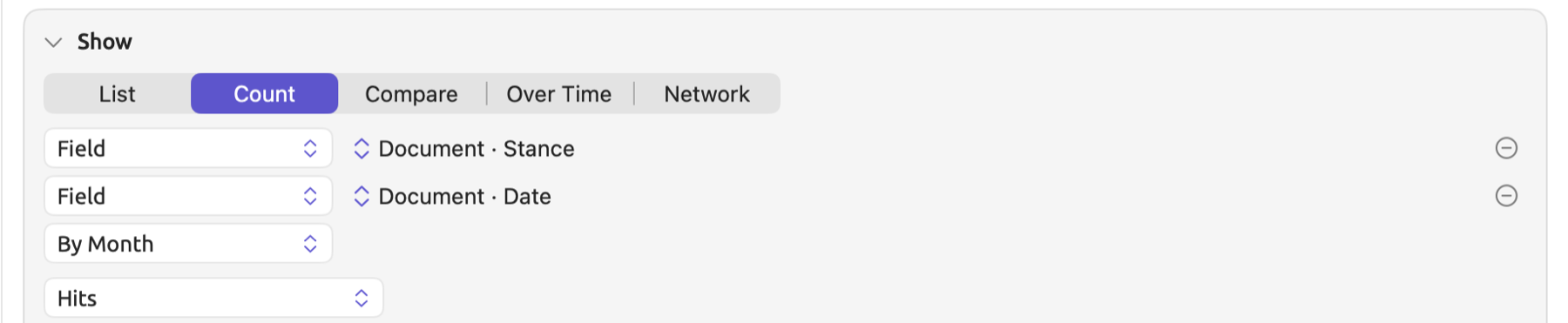
The rows are sorted based on the number they show, descendingly. Exceptions to this rule are rows for Position in Document, years, and months, which retain their natural ordering scheme. Within a table query result, rows and columns follow the order of the keys’ values, usually alphabetical.
Hits lacking any value for the key, such as the codings in “Heat Wave Report 2024” grouped by Group, appear under a No value row. A single hit featuring multiple values, such as a document featuring multiple tags, registers once under each of them. Consequently, the sum total of rows may exceed the actual hit count.
In Count and Compare, selecting Limit in the Show condition allows restricting the number of rows displayed. Its initial value is set to 50 and ranges up to 10,000 entries.
Measures
The menu showing Hits determines which number will be displayed in every row. This option is available for Count, Compare, and Over Time; Position in Document strips display single hits regardless of the choice. If the documents/groups compared vary in size (and they usually do), then Per 10,000 Words is recommended. Library units other than Documents offer only Hits and Share.
| Measure | Shows | Shown as |
|---|---|---|
| Hits | The number of hits | A whole number |
| Documents | The number of documents with at least one hit | A whole number |
| Per 10,000 Words | Hits for every 10,000 words of text | One decimal place |
| Coverage | The share of the text that the hits cover | A percentage with one decimal |
| Share | The row’s share of all hits | A percentage with one decimal |
Per 10,000 Words
Comparison of counts across texts with differing lengths is difficult. An occurrence of six hedges in a 600-word-long blog entry equates to a frequency of ten occurrences per thousand words, whereas six hedges in a text with 3,000 words become two occurrences per thousand words. A rate normalizes this comparison by dividing hits by word count, and then multiplying by 10,000 to provide more manageable numbers.
Here refers to hit count in the row, and to word count of the documents represented in the row. Word count uses the indexed text body minus punctuation. If the row refers to a document-level key, say “Stance”, then is computed using word counts in documents having the particular value. For all else, whether Code or Lemma keys, considers the sum total of word counts from all documents read by the query.
Suppose the three print documents in the “Skeptics” set are made up of 1,800 words containing 24 hedges. This gives a rate of . Meanwhile, the two online documents contain 1,200 words and 30 hedges. This leads to a rate of . On the other hand, for the “Skeptics” set Group By Code listing, which sums 3,000 words, the rate of a code having ten codings will be around .
The rate for the row combines hits and word counts from all the documents included. Long documents, thus, influence the resulting rate more than short ones. The rank test under Compare computes a rate individually for each document.
Documents get word counts during indexing only. Until a document is indexed, a word-based query ignores it completely, and the results bar shows the number of documents read. Any other unit besides words counts its hits even before the words are counted, giving artificially inflated rates.
Coverage
Coverage is a measure expressed in characters:
refers to the total number of characters that are covered by at least one hit, while is the total number of characters in the documents represented by that row, similarly selected as those for Per 10,000 Words. Characters where hits overlap are counted once.
For instance, consider “Running Out of Time”, a document comprising roughly 5,000 characters, and suppose it features three “Fear” codings of 150, 250, and 200 characters respectively, the latter two overlapping by 50 characters. The total number of covered characters would thus be , resulting in coverage of , or 11.0%.
Coverage suits codings best because it expresses what proportion of your texts you coded with the particular code. For words, Coverage yields proportions of covered characters, which are hardly useful in most cases.
Share
Share calculates the proportion of the row hits in relation to the total hit number within the scope of the query. For example, if the “Activists” set has 54 codings and 7 of them are “Fear” codings, the “Fear” row would have a calculation of . If some hits fall within multiple values, the sum may exceed 100%.
Drilling down
Each number in your counts reflects hits, and those hits can be opened as lists.
- Click a row in a Count or Compare list, a cell in a table, or a point in an Over Time line chart. The results area lists the hits behind that value in document order, as a concordance for passages, or as a table of records when Find is a Library unit such as Documents. The results bar names the value. A cell of the table from the Dictionary Categories by Document recipe, for example, gives Let’s Not Panic · Shields.
- Double-click a hit to open it in its document.
- To go back, click the × beside the value’s name. The count returns at once.
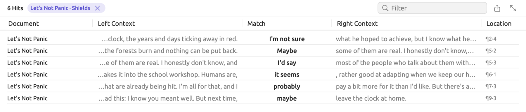
There is no consideration of the Limit in the Show condition while creating a drill-down list. However, any Limit defined in the Options condition is considered. If you modify any part of the query, your drill-down process stops immediately. During your drill-down list session, Export allows you to export the current list, whereas the Actions menu acts upon the hits within the list, such as creating a set of the documents they come from (see Chapter 18, Using Query Results). With regard to line charts, whenever there is a second Group By key and you click anywhere within the chart, it creates a list with the hits of all lines in that position.
To get passages for collocates or keywords, use the Concordance recipe.
Comparing groups
Compare works like Count but also incorporates testing differences between groups.
Running a comparison
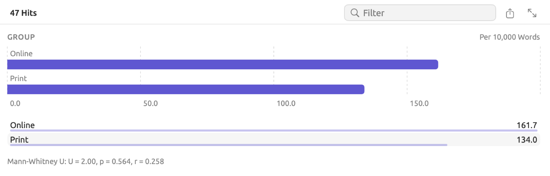
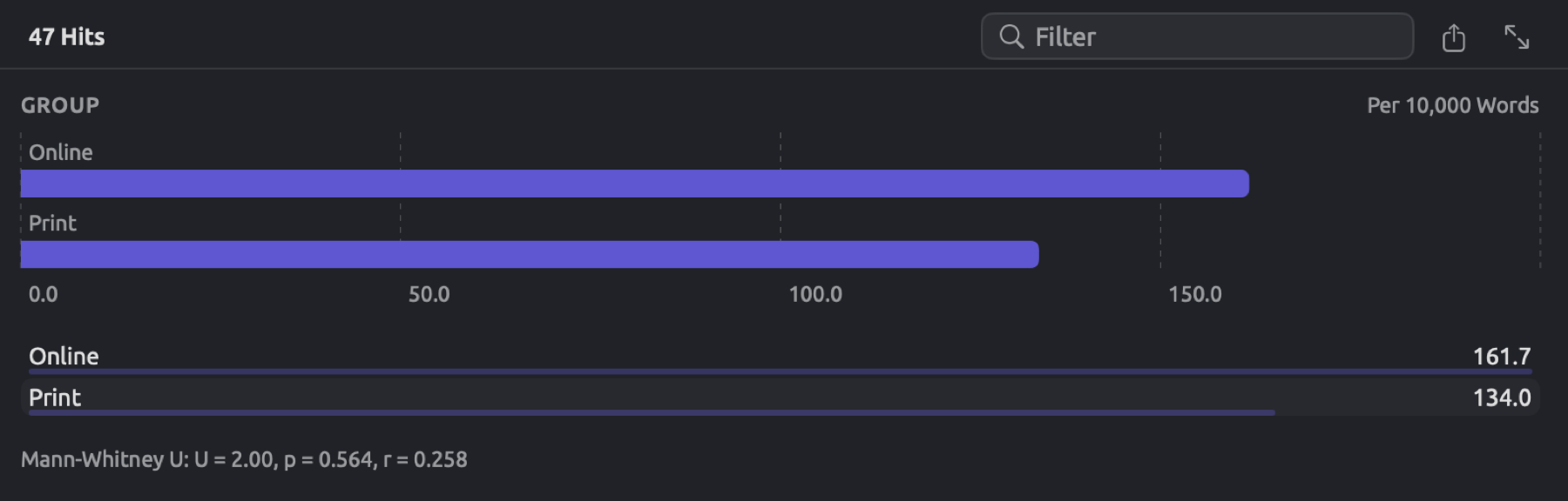
In “Climate Debate”, the five documents in the “Skeptics” set come in two groups called “Print” and “Online”. Additionally, this project contains a dictionary, “Hedges”, of words like perhaps, which soften claims. In particular, comparing the usage of these hedges per 10,000 words by group asks whether skeptics hedge more online than in print. For the figure, the query finds Text Matches with the menu showing Dictionary and “Hedges” chosen in the menu below it.
For comparing groups of documents:
- In Show, choose Compare.
- Click Group By.
- In the new row’s field menu, choose a property of the documents, such as Group or an attribute.
- In the menu showing Hits, choose Per 10,000 Words.
- Leave the menu showing Automatic as it is, unless one of the other tests below suits your question better.
In the example, the rows show pooled rates of 161.7 for “Online” and 134.0 for “Print”. Underneath the rows, a line gives the test result, here Mann-Whitney U: U = 2.00, p = 0.564, r = 0.258. The online documents hedge slightly more. p-values and effect sizes below describes the meaning of the numbers in detail. Test lines are darker with p-values lower than 0.05 and gray with higher values. You can select the text of a test line and copy it.
If Compare uses one Group By key, the test needs a document-level key. Document-level keys consist of Language, Project, and the document fields (such as Group, Date, or an attribute). Although Document is also a document-level key, the groups it forms contain only one document, hence making the test line meaningless, so read those rows by eye. With keys like Code, Lemma, or Position in Document, Compare only displays the numbers; those keys group hits within documents, and not whole documents. When there are no keys for grouping, Compare displays only one number. With two keys, the test works on the table instead (see Tests in a table later in this chapter).
Here is what each test in the menu showing Automatic does:
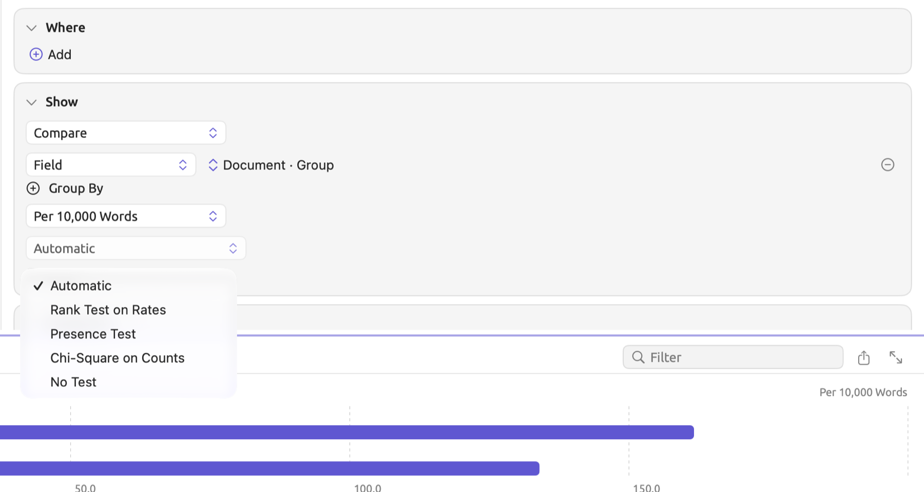
- Automatic selects the Presence Test if the measure is Documents and the Rank Test on Rates otherwise. Automatic is suitable for most cases.
- Rank Test on Rates compares the rates of the documents in each group. It performs the Mann-Whitney U test if comparing two groups and the Kruskal-Wallis H test if comparing three or more.
- Presence Test compares whether the number of documents with at least one hit differs between the groups. If comparing two groups, the test uses Fisher’s exact test; when there are more, it uses a chi-square test.
- Chi-Square on Counts compares the number of hits and total words per group with every word serving as an observation.
- Finally, No Test shows the rows alone without the test line.
When interpreting test results, bear in mind the following considerations:
- First, the test does not consider the numbers displayed in the rows. The rates of the documents form the basis of the rank test, while the presence test counts documents with and without hits. When dealing with a query looking at Words, Pattern Matches, Sentences, Paragraphs, Text Matches, Phrases, Noun Chunks, or Findings, or when the measure is Per 10,000 Words or Coverage, the rate becomes the number of hits divided by the number of words in each document. In any other case, such as Codings with the measure at Hits, the rank test divides by the number of characters in each document instead. Chi-Square on Counts has no words to compare in those cases and yields χ² = 0.00 and p = 1.000, which are meaningless figures. You should set the menu showing Hits to Per 10,000 Words before reading the rank test or Chi-Square on Counts. Apart from that, the measure affects only the choice made by Automatic.
- Second, all groups are included, even those that Limit or the Filter field hides.
- Third, documents missing a key value form their own group, No value, included in the comparison even when no row is displayed for them because they have no hits. In the “Climate Debate” project, “Heat Wave Report 2024” and “Carbon Tax Debate” fall into no group. Thus, grouping with the Group field at the project level will result in comparison among three groups. Comparison excluding documents without a value must be performed in a set that holds only the documents with a value.
- Fourth, documents taking several key values, such as tags, will appear in each group accordingly. The tests assume that each document belongs to one group. Choose keys taking one value in each document, such as a Picker attribute or the group itself.
p-values and effect sizes
Document groups rarely have precisely equal rates even when nothing sets them apart. The test will thus provide the likelihood that the difference could occur purely randomly and the size of that difference itself.
The p-value measures how likely the observed difference, or a larger one, could arise solely due to chance should no differences truly exist among the compared groups; it ranges between 0 and 1. A p-value of 0.04 implies that chance alone would yield such a result in about 4 of 100 comparisons. Various disciplines consider results significant if p < 0.05. A p-value is not the probability that a difference exists, and a p > 0.05 merely indicates insufficient evidence; often, the sample size is insufficient.
The effect size measures the difference between the groups according to some standardized metric. Effect sizes do not grow with increasing sample sizes, whereas p-values depend both upon the effect size and the number of observations. For several hundred documents, it is conceivable for a difference to reach statistical significance at p < 0.05 regardless of the triviality of that difference. Common rules-of-thumb for interpreting effect sizes r, φ, and V suggest 0.1 is small, 0.3 is medium, and 0.5 is large. Since ε² works on a squared scale, read 0.01, 0.09, and 0.25 as small, medium, and large.
In test lines, the type of hypothesis test used for comparing document groups appears along with the value for the test statistic, p-value, and effect size. A test statistic refers to a number generated by the hypothesis test based on the inputted data; the examples here include U-statistics, H-statistics, and χ²-statistics. Some test lines give extra information beyond the test statistic, specifically degrees of freedom (df, described in Rank test for three or more groups below). When the p-value is smaller than 0.001, the test line uses p < 0.001.
Rank test for two groups
The rank test examines whether the rates of the documents in one group tend to be higher than those of the documents in another group. Rank tests rely solely on rate rankings, not magnitudes; thus, having one document with a very high rate will not always sway results in favor of its group. In cases where you compare two groups, this test is known as the Mann-Whitney U test.
In this example, the numbers are invented so that calculations become simpler. Suppose the “Skeptics” set includes 3 print articles and 2 online articles, with every article totaling 600 words, including these hedges:
| Document | Group | Hedges | Rate | Rank |
|---|---|---|---|---|
| Net Zero Will Cost You | 3 | 50 | 1 | |
| The Models Keep Missing | 6 | 100 | 2 | |
| Who Pays for the Transition | Online | 12 | 200 | 3 |
| Science Is Never Settled | 15 | 250 | 4 | |
| Let’s Not Panic | Online | 18 | 300 | 5 |
The test begins with three steps.
- Each document gets its own rate per 10,000 words, such as for “The Models Keep Missing”. A document without hits takes part with a rate of 0.
- All documents are ranked by rate, from 1 for the lowest to 5 for the highest.
- U counts how often one group comes out ahead. There are pairs of one print piece and one online piece. In 5 of them the online piece’s rate is higher; in one, “Science Is Never Settled” (250) against “Who Pays for the Transition” (200), the print piece’s is. U is the smaller of the two counts, so .
Alternatively, the count in step 3 could also be calculated using ranks:
Here and stand for the size of each group of documents that you are comparing against one another (2 and 3 respectively). Parameter refers to the sum of the ranks in the first group of documents, which would equal in this case (online pieces). The minimum rank sum of the two documents would be . Therefore, and consequently .
This statistic is now compared to what the value of the statistic would be due to randomness had there been no difference between the two groups of documents. Each of the groups would be expected to be better than the other in roughly equal proportions among the comparisons; hence, the value should be near . Its typical distance from this value is its standard deviation, denoted by , with
And stands for the total number of documents. Therefore, . The number of standard deviations by which the statistic differs from the expected average then equals
For values from chance alone, the distribution of this z statistic follows the bell-shaped normal distribution. Most values fall between −2 and 2, while few lie further out. Values at least away from 0, on either side, make up about 0.248 of the distribution, which is the p-value. Using a spreadsheet program, you can obtain this value using =2*NORM.S.DIST(-1.155,TRUE).
The effect size measures the ratio of the z-statistic to , the square root of the number of documents:
Here, means z-statistic regardless of sign. Effect sizes range from 0 (neither group tends to prevail) to values approaching 1 as one group dominates over the other. In a case where each document from the first group prevails over each document from the second group, the effect size would still stay below 1; for groups of 2 and 3 it would be about 0.77.
Your test line would thus read Mann-Whitney U: U = 1.00, p = 0.248, r = 0.516. Despite the large effect size and the online pieces having prevailed in five out of six pairs, p is greater than 0.05. Given just five documents involved in the test, a distribution that uneven would still occur by mere chance in about 25 of 100 comparisons. A similar pattern repeated over twenty documents in each group would yield an even smaller p-value.
Ties arise when multiple documents show identical values; tied documents, such as several with a rate of 0, are assigned the average of the ranks they’d receive, so two documents tied for ranks 1 and 2 both get 1.5. When a tie occurs between one document of each of two groups, it is counted as half of a pair to both sides. In LemmaLoom, ties lead to reducing σ slightly. The p-value comes from an approximation using the normal distribution. Treat it as a rough guide for small sample sizes (fewer than about ten documents per group); the exact p-value of this example turns out to be 0.40 rather than 0.248.
Rank test for three or more groups
In the case of comparing three or more groups, however, the rank test is known as the Kruskal-Wallis H test. This test checks whether the groups’ average ranks differ more than could be expected purely due to random processes.
Suppose that you wish to explore how hedges used in the “Wide Reach” smart set are distributed depending on their respective stance values. Setting Group By to Attribute ▸ Stance achieves that goal. Your query considers the six original documents, in pairs per stance value, with the following rates:
| Stance | Rates | Ranks | Average rank |
|---|---|---|---|
| Activist | 0, 20 | 1, 2 | 1.5 |
| Skeptic | 50, 300 | 3, 6 | 4.5 |
| Neutral | 120, 260 | 4, 5 | 4.5 |
Mean rank refers to the average rank within a group. In this case, with three stances and six total documents, the mean rank of all documents is . Assuming stance had no effect on ranking positions, each of the three groups would have approximately equal mean rankings around 3.5. Deviations away from 3.5 are quantified through H in the following equation:
denotes the total number of documents, denotes the number of documents in group , while refers to the group mean rank. stands for “add up the following for every group”. The term is squared since squaring equally weighs deviation magnitudes regardless of whether they exceed or fall short of 3.5, and each is then multiplied by the corresponding number of documents. The factor in front scales H for a chi-square distribution.
With three stances:
If there were documents having a common rate, the statistic above would need to be corrected by dividing it by , where each refers to how many documents share a particular rate. Had 2 documents shared one rate out of the total of six, then this correction term would be . If there weren’t any ties, the correction factor would simply be 1.
The statistic based on chance alone follows the chi-square distribution. What defines such a distribution is how many degrees of freedom it has. Here, it is one fewer than the number of groups because knowing all the others allows one to know the last average rank value. Thus, with 3 groups, the df=2. The p-value is essentially the probability of getting a value as extreme as the observed one or greater by chance alone. With two degrees of freedom, the p-value equals , where is the exponential constant, about 2.718 ( is the base of natural logarithms, and a calculator button computes any power of ). Hence, in this case, . Alternatively, in a spreadsheet, one could calculate this probability using the formula =CHISQ.DIST.RT(3.43,2); the function works for any df.
The effect size is defined as follows:
If all average ranks are equal, then this effect size would be 0. It increases toward its largest potential value of 1 as the separation of the groups grows.
The Kruskal-Wallis H test line reads Kruskal-Wallis H: H = 3.43, df = 2, p = 0.180, ε² = 0.686. The two activist texts hedge the least. While this effect size is quite large, there is insufficient evidence to reject chance in light of only six total documents. Even in the event of getting a very low p-value, the result only implies the existence of a difference; look at each row individually to discover which groups are higher.
Chi-square on counts
Chi-Square on Counts assumes one observation per word in each group. So, each word either is a hit (1) or is not (0). This test happens to be very common in many corpus linguistics papers, and is useful when comparing against previous work.
Here’s the table you’ll get for the example in the “Skeptics” set:
| Hedges | Other words | Words | |
|---|---|---|---|
| Online | 30 | 1,170 | 1,200 |
| 24 | 1,776 | 1,800 | |
| Total | 54 | 2,946 | 3,000 |
Under Hedges and Other words lie four cells that comprise the contingency table; the Words column and the Total row show their sums. Assuming no effect due to the medium upon the number of hedges, the count of hedges within a particular cell would bear proportionality to the number of words in its respective row. Each cell has an expected count, calculated using the row sum multiplied by the column sum divided by the grand total. Expected counts would therefore come out as for online hedges, and similarly 32.4, 1,178.4, and 1,767.6. In general, the formula for calculating the test statistic (chi-square; χ is the Greek letter chi) is:
in which denotes the observed count whereas denotes the expected count within each cell individually. The summation extends to all cells within the contingency table. Squaring each term ensures only positives even in cases wherein the difference between observation and expectation goes negative. Dividing each squared term by provides emphasis on differences according to magnitude relative to , so a difference of 8.4 weighs more heavily in smaller cells than in larger cells. For instance:
This results in approximately 3.267, 2.178, 0.060, and 0.040 respectively, making . Degrees of freedom (df) for a contingency table amount to (number of rows minus 1)(number of columns minus 1); thus, this table has 1 degree of freedom (). The chi-square distribution table for df=1 is as follows:
| χ² at least | p at most |
|---|---|
| 3.84 | 0.05 |
| 6.63 | 0.01 |
| 10.83 | 0.001 |
When the χ² statistic equals 5.54, it falls somewhere between 3.84 and 6.63, so p falls between 0.05 and 0.01. Calculating =CHISQ.DIST.RT(5.54,1) shows that p=0.019. To calculate the effect size with the Cramér’s V statistic, use the equation:
where denotes the grand total, and represents the number of rows or of columns in the table, whichever is lower. With two rows and two columns in this table, and . Consequently, the result equals . Thus, the test line is Chi-Square: χ² = 5.54, df = 1, p = 0.019, V = 0.043.
Recall that with the same invented counts, the previous rank test produced p=0.248. The current test produces p=0.019. These probabilities are different since both methods are different; namely, the rank test takes into account five documents, whereas this test analyzes 3,000 words as separate observations. Because authors exhibit patterns and topics come in clusters, words that occur within a text aren’t independent from each other, meaning this test tends to produce a p-value that is too small when texts differ among themselves, which almost always happens. This is precisely why Automatic favors a rank test over this method.
Given that hedges account for a negligible share of the word count, V will be very close to 0, as it would for nearly any word. Interpreting V statistics is relatively meaningless for this test specifically.
Presence test
The Presence Test examines if the share of documents containing hits is greater for one group over another. If the measure is Documents, then Automatic chooses the Presence Test; use it when you care about presence rather than frequency counts. The Presence Test uses Fisher’s exact test for two groups, calculating every possibility without approximation.
For the example of “Climate Debate”, the query examines “Deadlines”, the subcode of “Urgency” for target years or deadlines. The query looks for differences between print and online skeptic articles regarding the presence of deadlines, regardless of the number. This means setting the measure to Documents because a single instance is enough. The Codings included here come exclusively from the document set of “Skeptics”, filtered on the code “Deadlines” in the Where condition, and the results are grouped by Group.
To perform the presence test:
- Set up a comparison as described in Running a comparison earlier in this chapter.
- In the menu showing Per 10,000 Words, choose Documents.
These numbers come directly from the statistics in the project itself. Of the three print documents, one has been coded with a “Deadlines” code, while the two online documents both have a “Deadlines” code.
| With a “Deadlines” coding | Without | |
|---|---|---|
| 1 | 2 | |
| Online | 2 | 0 |
Fisher’s test makes the assumption that the marginal sums are fixed, which implies that the total number of documents is fixed at 5, the total number of print pieces is fixed at 3, and finally, the total number of coded “Deadlines” documents is fixed at 3. Given the assumption above, if there were no effect from the medium, the coding would fall on 3 documents chosen randomly from the 5 available. The number of ways that items may be chosen from among possibilities is denoted by ; for example, , indicating that you have 6 combinations to choose 2 objects from four possibilities. Calculating the combinations entails dividing the multiplication of descending natural numbers beginning with by the multiplication of ascending natural numbers beginning with 1 (). Hence . In spreadsheets, calculating may be done using =COMBIN(5,3), returning 10.
Out of the total three documents coded, precisely documents will be among the print documents in combinations, that is, selected from three print documents times from the two online documents.
| Print pieces with a coding | Ways | Probability |
|---|---|---|
| 1 | 3 × 1 = 3 | 3/10 = 0.300 |
| 2 | 3 × 2 = 6 | 6/10 = 0.600 |
| 3 | 1 × 1 = 1 | 1/10 = 0.100 |
There cannot possibly be zero print pieces with a coding since there are only two online pieces. The observed split, one print piece, has the probability 3/10. The p-value adds up the probabilities of every split no more likely than that, here one print piece (3/10) and three (1/10), so .
The test line is Fisher’s Exact Test: χ² = 2.22, df = 1, p = 0.400, φ = 0.667. The chi-square value is the same statistic calculated from the above 2x2 table, provided solely for reference purposes; the p-value is Fisher’s. Phi is the Cramér’s V effect size for a table of 2 rows x 2 columns, . By the rule of thumb, this effect size is considered substantial. However, five documents are again insufficient to achieve significance.
When read off the distribution of the chi-square test statistic, a value of χ² = 2.22 corresponds to a value of p ≈ 0.136. This is about a third of the value from Fisher’s exact probability method, which gives 0.400. However, expected counts must be greater than approximately 5 for a good fit with the chi-square distribution. In this case, they are only for print pieces with a coding, and 1.2 without, and similarly with and 0.8 without for online pieces. Fisher’s calculation counts the possibilities exactly.
When there are more than two groups, the presence test becomes the chi-square test using an analogous table of groups versus documents with and without hits. As usual, Cramér’s V measures effect size. No test line is shown whenever all or none of the documents contain hits.
Tests in a table
Compare with two Group By keys yields a table, whose test is the chi-square test of independence based on cell counts. This test enables you to determine whether or not two properties are related in your collection, such as “Stance” and group. The expected count of a cell is once again the product of its row sum and column sum, divided by the grand total number of observations in the table, with the rows containing no hits removed.
Automatic selects the chi-square test only for queries where Find is Documents or another Library unit, so that each hit represents a distinct entity. For passage-level queries it selects no test due to the non-independence of observations coming from the same document. Testing the resulting table anyway requires selecting either Chi-Square on Counts or Presence Test. Both options return the chi-square statistic for cell counts. Rank Test on Rates returns no test for a table.
For tables with more than two rows or columns, Cramér’s V will be calculated using the smaller of the two dimensions. An example table consists of 3 rows and 4 columns, with a grand total of 60 observations and . Thus, , and .
Choosing a test
| Question | Measure | Test |
|---|---|---|
| Do the documents of one group use something more often? | Per 10,000 Words | Automatic (rank test) |
| Do more documents in one group use it at all? | Documents | Automatic (presence test) |
| How do my figures compare with corpus studies that test word counts? | Per 10,000 Words | Chi-Square on Counts |
| Are two document properties related, such as “Stance” and group? | Find Documents, two Group By keys | Automatic |
Over time
Over Time illustrates the distribution of hits along something with an order. This could be positions within each document, elapsed minutes of recordings, dates of documents, etc. Selecting Over Time in a query without specifying a Group By key adds Position in Document, with one strip per document; with other keys, graphs take the form of line charts.
Where hits fall in each document
The strips allow you to interrogate issues of the text structure; for instance, whether a theme occurs at the beginning or end of a piece. Additionally, the strips allow you to determine if it occurs in every document in your set, or only occurs in a handful of documents in the set. Taking “Climate Debate” as an example, you might inquire where fear occurs in activist texts. The figure shows the “Fear” codings of the “Activists” set, found with a rule on Code in the Where condition.
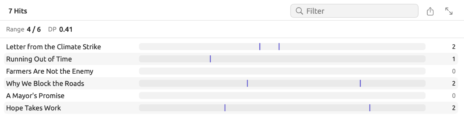
Each document the query reads will be presented with a row showing its title, strip, and number of hits. The strip is an illustration of the occurrence of hits in the document from its start (on the left) to its end (on the right); each hit shows up as a small tickmark at the position where it starts. Documents that contain zero hits show an empty strip and a count of 0.
Above the strips is listed Range, which gives you the number of documents containing at least one hit among all documents processed, e.g., 4 / 6. The statistic deviation of proportions (DP) measures how evenly the hits are distributed among documents relative to their sizes:
Here, refers to the count of hits in document , and to the total count in all documents. Similarly, refers to the size of document and to the size of all documents. Size refers to the number of words processed in documents when analyzing words, or when the measure is Per 10,000 Words or Coverage (refer to Running a comparison earlier in this chapter). Otherwise, as in Codings with the measure set to Hits, it refers to the character count of the documents. Shares tend to be almost identical in both cases. The former fraction shows the document’s proportion of hits, whereas the latter shows its proportion of all text analyzed. The two vertical lines around the fractions imply taking their absolute difference (that is, “the distance between” them, ignoring their signs).
Consider a set with three documents of size 500, 500, and 1,000 words respectively, containing 2, 0, and 2 “Fear” codings. As proportions of text, those documents represent 0.25, 0.25, and 0.5; and proportions of hits, 0.5, 0, and 0.5. Thus,
and Range equals 2 / 3. A DP equal to 0 signifies an exact proportional distribution of hits. DP closer to 1 means clustering in small parts of the text. Note that DP measures hits’ proportions across documents, regardless of their location within each document; see their positions on the strips, or alternatively use Count with Group By Position in Document, which pools all documents into one row for each tenth that has hits, from 0–10% to 90–100%.
Trends over dates and recordings
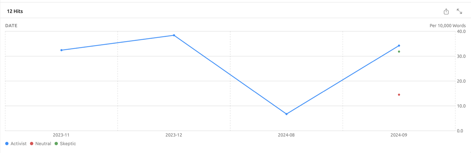
If your key is a date field, Media Time, or any other ordered key, then Over Time uses a line chart. Adding an additional Group By key gives you lines for each value, which appear with a legend underneath the chart. Hovering the mouse pointer over the chart reveals values at that point, while clicking lets you drill down to its hits.
All documents in “Climate Debate” have a Date field, thus allowing you to track the “Fear” codings during each month of the debate, with each line representing one stance. The measure is Per 10,000 Words.
To create a line chart over dates, follow these steps:
- In Show, choose Over Time. A key row with Position in Document appears.
- In that row’s menu showing Position in Document, choose Field.
- In the field menu beside it, choose a date field, such as Date.
- In the menu showing Each Value, choose By Year or By Month.
- For one line per group, click Group By, and choose the second key in the new row’s field menu, such as Attribute ▸ Stance.
- In the menu showing Hits, choose Per 10,000 Words.
The Speaker Turns over Time recipe detects Speaker Turns and bins them according to Media Time and then the Speaker field. This recipe appears when your current scope includes audio or video documents. Each point counts the speaker turns beginning within each minute of the recording, labeled 0:00, 1:00, and so forth. For the “Radio Debate”, there will be one line each for the “Host”, the “Activist”, and the “Skeptic”.
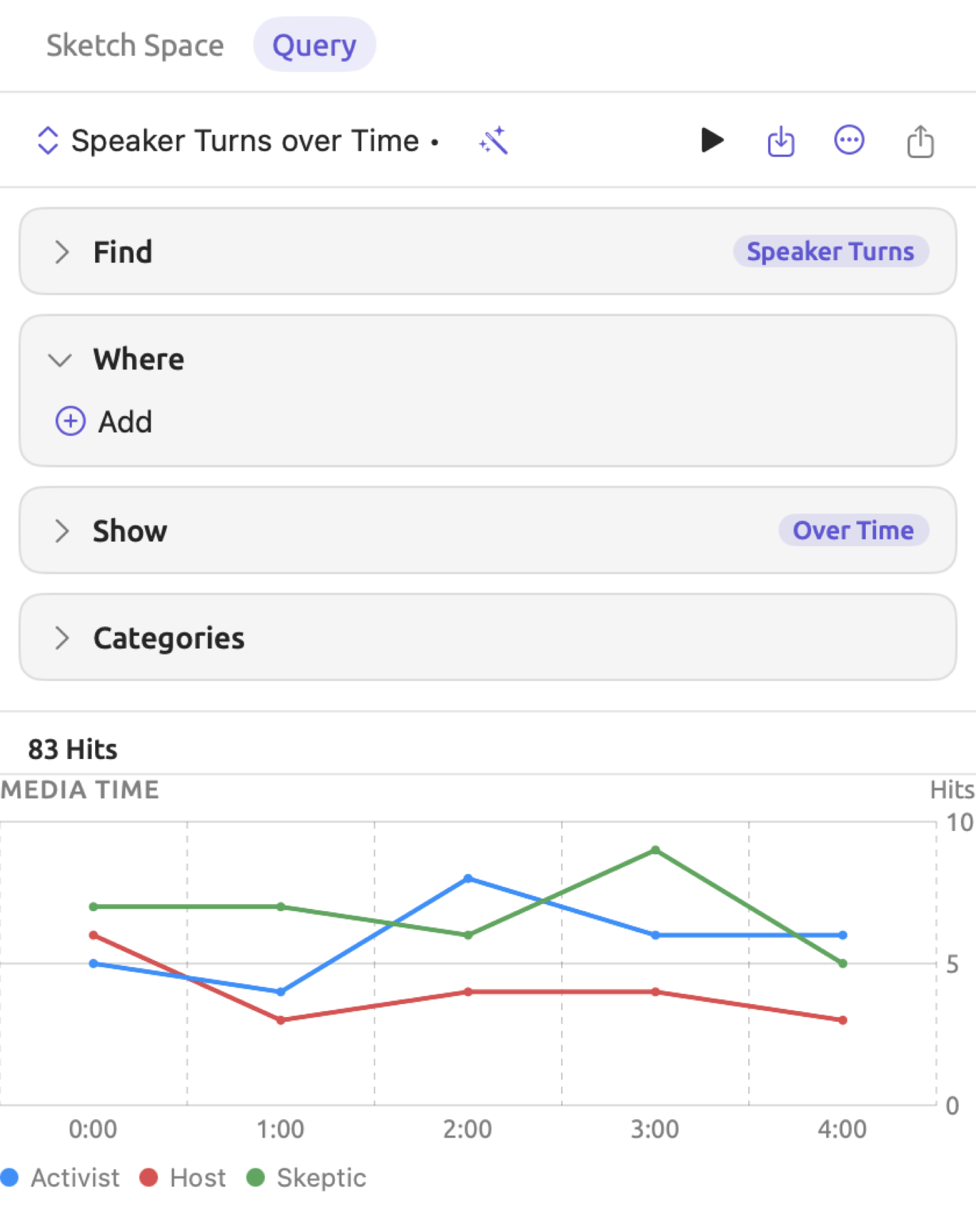
Per 10,000 Words and Coverage divide by the text of the documents each row covers. So when you specify Date, the text is that of the documents from that year or month. With Media Time and Position in Document, it is the text of all documents read, which means the line’s shape matches that of Hits; use Hits there.
Collocates
The collocate list is a listing of words that appear in proximity to a hit more often than what would be expected based on the word’s global occurrence. Some examples for the lemma climate in the sample project “Climate Debate” could be policy, science, and crisis. Consider the collocate list to be an abstract representation of a word’s associates. Use it to investigate the usage of a word throughout many documents or to identify phrases worth close inspection.
Making a collocate list
The figure presents the collocates of climate in the project “Climate Debate”, sorted based on logDice scores.
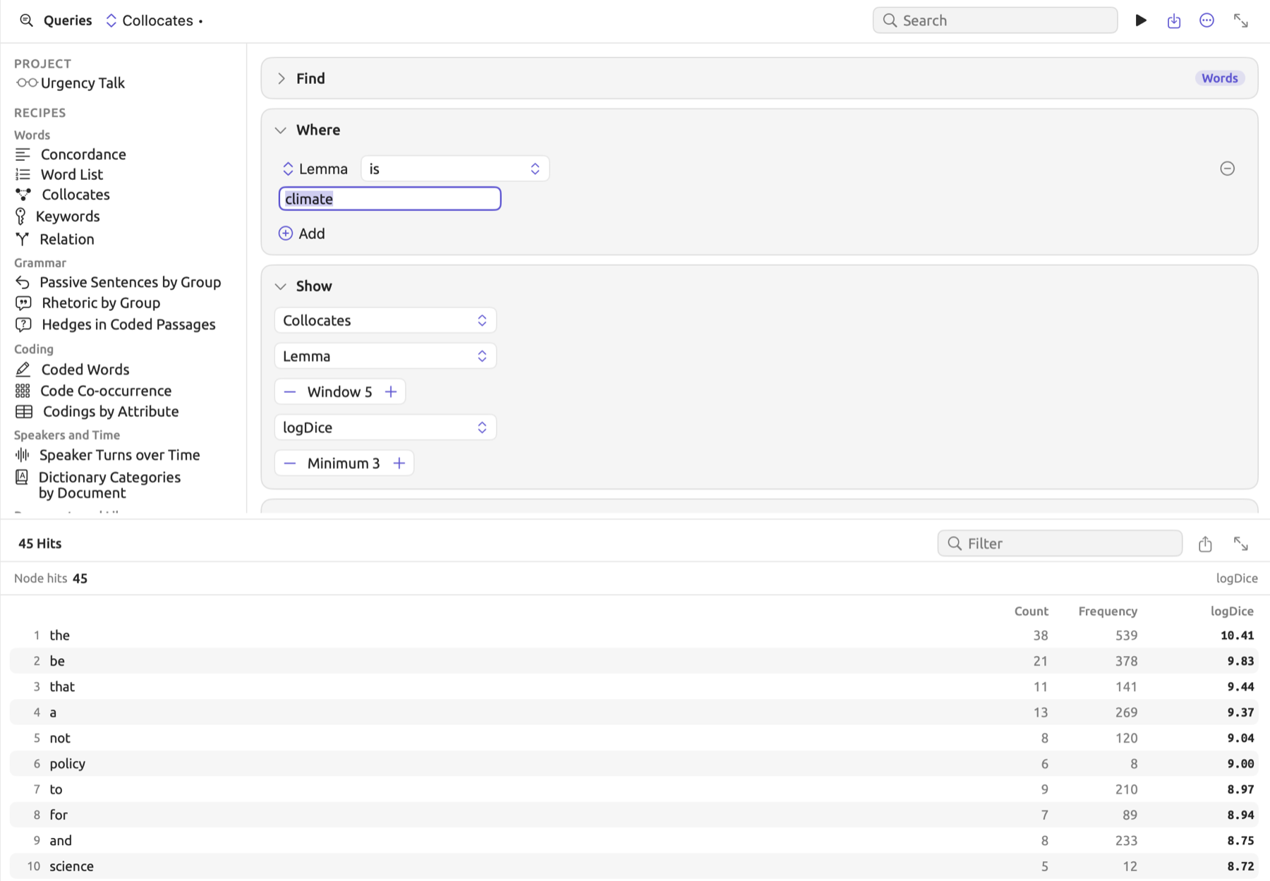
For making a collocate list:
- Open the Queries section of the set or project.
- Under Recipes in the left column, click Collocates. The recipe finds Words whose Lemma equals a value.
- In the Where condition, enter the lemma you are interested in as the value.
Adjust the settings in the Show condition if you need to:
- The menu showing Lemma decides which items should be counted, whether that be lemmas (Lemma), separate words regardless of capitalization (Word), or word classes such as NOUN and ADJ (Word Class), depending on your preference.
- The Window determines how many words ahead and behind each hit will be examined; it may range between 1 and 10 with the default being 5.
- The menu showing logDice defines which association measure the collocates will be ranked by; the default is logDice.
- Minimum indicates the minimum frequency with which an item must appear alongside the hits for it to be included; it may range between 1 and 50 with the default being 3.
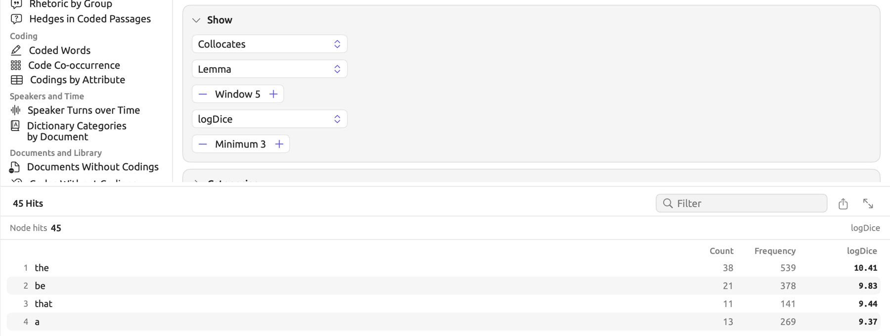
In each document’s Query facet is a Recipes menu located in the bar at the top. The Collocates recipe can be found in it; the menu shows an icon resembling a magic wand.
A table displays the results, showing each word alongside its Count (occurrences next to hits), Frequency (number of occurrences in the documents searched), and finally the association score calculated according to your settings. The table is sorted by the scores, highest first, with 200 entries being displayed at most by default. Above the table, Node hits displays how many hits were selected for collocation (in corpus linguistics terminology, the node refers to the searched word). Count and Frequency values are displayed below each word in the inspector.
For each hit, the surrounding words will be collected up to the Window number on each side, within the same sentence, ignoring any punctuation marks along the way. Words belonging to the hit itself are not considered. If multiple hits occur in close proximity to each other, then overlapping words are counted separately with respect to each hit.
Collocation requires positional information of each hit among the words, which Text Matches provide exclusively when the text row’s first menu shows Word, Word Form, or Lemma and its second menu shows Terms or Dictionary. Otherwise, as with matches on Text or by Regular Expression, no hits can be used in calculating collocates, and the list is empty.
The association scores
Each of the seven scores starts with the calculation of four variables. Taking policy near climate again as an example, suppose the following:
- is the Count value, the number of times the word appears in the windows.
- is the sum of the lengths of the windows. Forty-five hits with five words on each side would give 450, but hits near the start or end of a sentence have shorter windows.
- is the Frequency value, representing how many times the word occurred in the whole project.
- is the number of words in the project.
If policy were randomly distributed, the windows, which hold 360 out of 9,000 words, would get the same share of its 10 occurrences. Hence, the expected count would be:
Many of these scores employ logarithms as part of the calculations; the logarithm represents the exponent of powers of 10, or any other base, required to reach the value. The logarithm of 1,000 with base 10, for instance, is 3 (), while the logarithm of 8 with base 2 () would return 3 since three doublings reach eight. The natural logarithm, written , asks the same question about the number (about 2.718) and can be computed via the ln button on calculators. For all three, the logarithm of 1 is 0, numbers above 1 have positive logarithms, and numbers between 0 and 1 have negative ones. The log base two of 8 can similarly be achieved by dividing by .
| Score | Formula | policy | the |
|---|---|---|---|
| MI | 3.91 | 0.89 | |
| MI3 | 9.08 | 11.53 | |
| T-Score | 2.29 | 2.91 | |
| Z-Score | 8.85 | 3.96 | |
| Log-Likelihood | see below | 25.58 | 14.22 |
| Dice | 0.03 | 0.09 | |
| logDice | 9.05 | 10.51 |
The column for the assumes it occurs 40 times in the windows and 540 times in the project, so the expected count would be . In the table above, both columns show how differently the scores rank a specific partner (policy) and a very common word (the).
MI (mutual information) measures how many doublings, or bits, the observed frequency lies above the expectation . In the case of policy, , meaning that it appears fifteen times as much as one would expect if the distribution was purely random; bits, slightly less than four doublings. MI prefers less frequent partners. A word occurring just once in the entire project, next to climate, would yield an expectation of , and a score of around 4.64, greater than policy itself. Minimum keeps such uncommon words out of the list.
MI3 raises the observed count to the third power before division. This increases the weight given to common pairs. Here policy yields a score of , and the ranks higher.
T-Score calculates the ratio between observed minus expected over the square root of the observed. For policy, this gives . T-Score increases with the observed count; it favors high-frequency collocates. Corpus linguists tend to consider a value of 2 a rough sign of association beyond chance.
Z-Score calculates the ratio of the same difference but relative to the square root of the expected count, here . The low expected count in cases of rare words results in extremely high z-scores.
Log-Likelihood, explained in How the two scores are calculated later in this chapter, tests whether the counts are significantly different from their expectations using a statistic derived from the logarithms. Its calculation involves setting up a contingency table with the observed frequencies and calculating the expectation based on row and column sums, just like in the chi-square test presented in Chi-square on counts earlier in this chapter. For policy, the four counts are policy in the windows (), the other words in the windows (), policy outside the windows (), and all remaining words (). Each cell would thus have a corresponding expected frequency, namely 0.4, 359.6, 9.6, and 8,630.4. Finally, the log-likelihood value is as follows:
With regard to the policy example, the value is . Log-likelihood tests are used to estimate the statistical significance of deviations from chance expectations based on the same threshold criteria as chi-square test statistics; p-values less than 0.05, 0.01, and 0.001 correspond to values above 3.84, 6.63, and 10.83 respectively. With regard to keyword lists, only the two components relevant to the word itself, and , are required.
Dice pits the joint count against both margins, and computes a score of for policy. Only when all window words are occurrences of policy will Dice equal 1, and vice versa. logDice is the Dice index transformed to a maximal value of 14, giving for policy. logDice decreases its score by 1 upon halving Dice, and increases its score by 1 upon doubling Dice. As logDice pays no heed to the size of a set, it makes sense to use logDice whenever set sizes vary. Furthermore, in smaller sized projects like “Climate Debate”, logDice ranks frequent words like the high.
Use logDice for a balanced list, MI with a higher Minimum for rarer partners, T-Score for the most frequent company, and Log-Likelihood for the strongest evidence. Before relying on a collocate, list its passages with the Concordance recipe.
Keywords
A keyword list indicates the words which a collection of documents has used noticeably more or less often than another collection of documents. The purpose here is mostly exploratory, discovering something interesting about your documents before you decide what to code or which words to follow up. In “Climate Debate”, a keyword list for activists when compared against skeptics may include we, hope, and children, the words used more often by activists. Conversely, words like model and about may appear among the words used less often. By looking at concordances of these interesting words, you discover why they stand out. The Concordance recipe locates those passages which include these words.
In LemmaLoom, the difference between two collections of text is calculated relative to the target, the set of documents your query covers, and the reference, what you compare it with (the rest of the project, another set, or the whole project).
Making a keyword list
Keyword lists are usually produced for a set, either within the Queries section of the set, or within Window ▸ Queries if you select your set as the scope. In order to generate a keyword list for a single document, put that document into a set of its own. The example project “Climate Debate” has separate “Activists” and “Skeptics” sets so that you may compare the vocabularies used by both activist and skeptic sides.
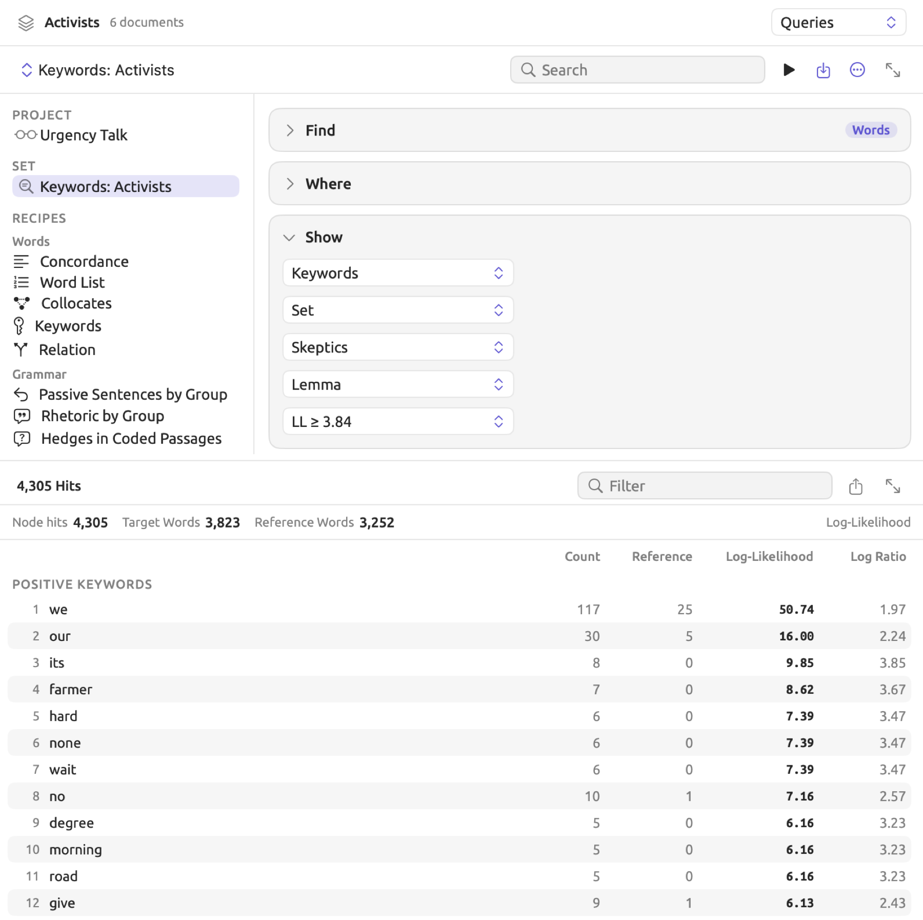
For creating a keyword list:
- Open the set and click Queries.
- Under Recipes in the left column, click Keywords.
In the Show condition, choose a reference in the menu showing Rest of Project:
- Rest of Project pertains to measuring the target in relation to the rest of your project. This should be run if all documents in your project share a common language; otherwise, the reference will mix languages too, and thus, a comparison with Set is recommended, where you can choose a set of documents in the target’s language.
- When you choose Set from that menu, the next step is selecting another set to compare with the target from the menu that appears. The results area shows No set chosen until you choose another set. Selecting the set the keyword list was generated from yields Nothing to compare with. Documents that belong to both sets are double-counted.
- The Whole Project comparison measures the differences between the target and the entire project, including the target itself, which means that the differences returned tend to be somewhat smaller than with Rest of Project. This comparison is useful when measuring multiple sets relative to one and the same baseline.
- In the menu showing Lemma, keep Lemma to count dictionary forms together (run, runs, and ran count as one word). Choose Word when a particular form matters; each spelling is then counted separately. Capitals are ignored either way.
- Leave the menu showing LL ≥ 3.84 as it is for now. It hides words whose difference could easily be chance (see How the two scores are calculated below).
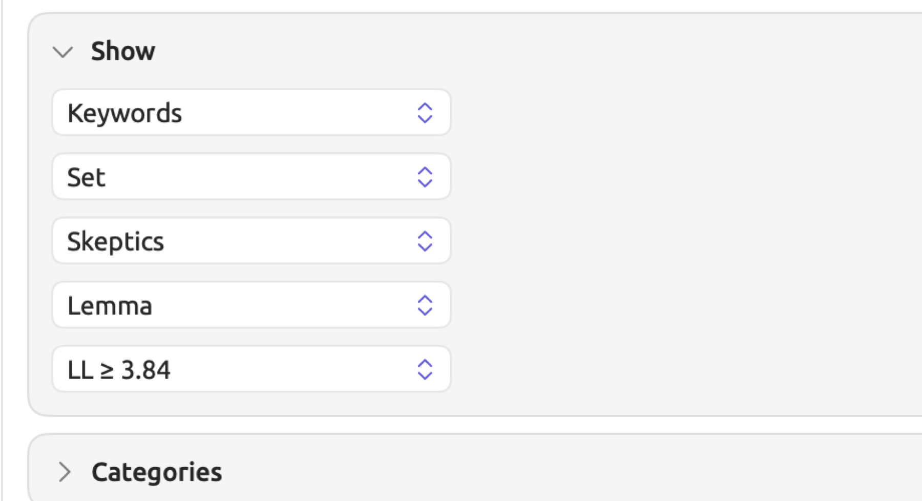
Like any other query you may run from the Queries section within your project, a keyword query there targets your whole project. As such, the menu showing Set offers only that one option, and the comparison is performed relative to whichever set you select. The Keywords recipe in particular only becomes available after creating a set in your project, and it defaults to selecting the first set within your project, but you can alter this choice from the menu showing that set’s name. Any keyword queries saved using another reference will automatically switch to Set as well upon being opened at project level.
All rules listed within the Where condition are treated equivalently on both sides of the comparison. If any rule filters out some common words, then these words will also be excluded from the reference side, meaning that whatever number appears above each list is the count minus the filtered-out words. For a rule to affect the reference, however, the reference documents must be searched as well. This makes the computation time greater than that with an empty Where condition.
Like the target, the reference follows Corpus in the Options condition, which determines which documents should be considered (original documents, translations, or both).
Under Positive Keywords, those words that occur more often in the target relative to the reference are listed, while under Negative Keywords, those that occur less often are listed. Each of the two lists is ordered by log-likelihood, highest first, and contains at most 200 keywords by default. Each row in the table includes:
- Count, how many times the keyword occurs in the target.
- Reference, how many times it occurs in the reference. Since the two document collections usually differ in size, these two counts aren’t directly comparable. Both scores will consider that imbalance in computing.
- Log-Likelihood, which shows how strong the evidence is that the frequency difference isn’t random. Both counts are used here.
- Log Ratio, how great the difference between the frequencies is.
Above the lists, Node hits shows how many words (including punctuation marks) the query found overall. Target Words and Reference Words show the number of non-punctuation words used in the target and reference document collections respectively.
Should the reference hold no indexed documents, there’s nothing to compare the document collection against. Hence, you get the message No matches in the results area.
Only keywords that occurred at least three times in their respective document collection (the target for a positive keyword, the reference for a negative one) qualify as candidates.
Numbers will be taken into account, while other characters such as punctuation and symbols won’t. Neither side will include documents that haven’t been indexed yet. Should that happen with the target side, the results bar displays a message showing how many of its documents were counted, such as 5 of 6 for the “Activists” set.
How the two scores are calculated
This ranking is based solely on log-likelihood values. Thus, a frequent word with a small difference can rank high, whereas an infrequent word with a large difference may not even reach the cutoff. At the end of this section, the words the and thermometer show examples of such situations. Look at both columns before you decide a keyword is worth following up.
Expected counts
Log-likelihood analysis involves comparing expected frequency counts with observed frequency counts. Due to the potential discrepancy between the sizes of the two collections, log-likelihood begins by computing expected frequency counts based on the assumption that the word makes up the same share of the text in the target and the reference. The formula used to derive the expected count is presented below:
Here, and denote the expected count for the target and reference, respectively. Meanwhile, and represent the occurrence of the word within the target and reference, while and denote their sizes in words, shown as Target Words and Reference Words; 1 always stands for the target and 2 for the reference. The fraction is the word’s share of all the text. For instance, consider the “Climate Debate” example where the target contains 3,000 words belonging to the “Skeptics” set and the reference contains 6,000 words from the rest of the documents in the project. In this case, the word about occurs 18 times within the target and 9 times in the reference. Thus, its total occurrence is 27, meaning it occurs about once every 333 words. Since the target represents one third of the entire 9,000 words, it would be expected to hold one third of the 27 occurrences and the reference the other two thirds (the expected counts), hence and .
Log-likelihood
Log-likelihood, abbreviated as LL in the menu showing LL ≥ 3.84 and represented numerically in the Log-Likelihood column, quantifies the deviation between observed and expected counts of a word in the two collections. It has an equation notation of ; the number 2 here does not indicate squaring. Rather, it is part of the name.
refers to the natural logarithm, described in The association scores earlier in this chapter.
In this formula, there are two components held by parentheses. They correspond to each of the collections. Each component represents a comparison between the observed and expected counts. When these values match perfectly, their quotient equals 1, its natural log equals 0, and the component thus contributes 0 to the sum. Observed and expected counts will always add up to the same total; for about, 18 + 9 = 9 + 18 = 27. This means that a word occurring more frequently than expected in the first collection implies fewer occurrences than expected in the second, and vice versa. So a deviation on the higher end contributes positively, while one on the lower end contributes negatively. In any pair, the positive part exceeds the negative one, which results in non-negative outcomes. Further deviation leads to greater increases in value.
Each of these logarithms is multiplied by its respective count, meaning that differences observed frequently contribute much more weight toward the score; thus, common words may acquire a high score relatively easily. The presence of 2 at the front, as well as in place of the base-10 logarithm, ensures that the formula’s output is scaled similarly to the chi-square distribution, the distribution which the threshold values come from. In cases where the count happens to equal zero, then that particular summand becomes nullified due to the fact that no log of zero exists.
For about, , which yields a natural log of around 0.6931; whereas , resulting in a natural logarithm of about −0.6931. Thus,
This calculation results in the value displayed in the column, 12.48.
By itself, the log-likelihood score tells little as to whether there is significance since counts also vary by chance. For instance, simply partitioning one collection randomly into two parts leads to each part using its words at varying frequencies, resulting in positive log-likelihood scores. The threshold hides words whose scores are likely due to mere random chance.
| Threshold | Share of words with no real difference that still reach this score |
|---|---|
| LL ≥ 3.84 | about 5 in 100 () |
| LL ≥ 6.63 | about 1 in 100 () |
| LL ≥ 10.83 | about 1 in 1,000 () |
These are the cutoffs of the chi-square distribution with one degree of freedom, while the denotes the p-value that has been discussed in p-values and effect sizes earlier in this chapter. At around 12.5, about surpasses all three cutoff values.
Keyword lists examine thousands of words simultaneously. If 2,000 of the words had no real differences, then approximately 100 of those (5 out of every 100) still make it past LL ≥ 3.84 while just 2 make it past LL ≥ 10.83. However, real differences in a large project are based on numerous occurrences and thus exceed these cutoff values by far, rendering a stricter cutoff negligible in cost.
Log ratio
The Log Ratio formula calculates the size of the difference between rates:
The numerator is the rate of use of the word in the target, whereas the denominator is that of the word in the reference. The logarithm denotes how many times the ratio doubles itself; means double usage by the target compared to the reference, whereas implies quadruple and implies eightfold usage. If equals 0, then both sides use it with equal frequency, while means that the target uses it half as often. As ratios without logarithms, however, “twice as often”, which equals 2, and “half as often”, which equals 0.5, will have unequal distance to 1. In contrast, log ratios put both at +1 and −1 respectively, equidistant from 0, so positive and negative keywords can be read on one scale.
In computing , every count has 0.5 added to it; this ensures that no zeroes occur in either the denominators or the argument of the logarithm, both being mathematically undefined.
Take the case of about:
Here, the target rate is , around 6 instances per 1,000 words. Meanwhile, the reference rate is , roughly 16 instances per 10,000 words. Dividing the former by the latter yields 3.89, lying somewhere between 2 (one doubling) and 4 (two), resulting in a Log Ratio of approximately 1.96. Thus, the skeptics use it almost four times as often as the remainder of the project.
Within the two document collections mentioned above, the appears 210 times in the target collection and 330 times in the reference collection; meanwhile, the expected counts are 180 and 360, respectively. It obtains a log-likelihood value of around 7.3, surpassing the two lowest thresholds, meaning the evidence for a difference is good. However, its Log Ratio of 0.35 is relatively low because the target collection uses it about 1.3 times as often as the reference.
Thermometer appears three times in the target document collection and once in the reference, against expected counts of 1.33 and 2.67, respectively. Adjusted based on both document collections’ relative sizes, the target uses it six times as much as the reference. With this in mind, its log ratio comes out to 2.22, greater than that of about; yet, it fails the lowest threshold due to its log-likelihood score being just 2.90, since the whole difference rests on four occurrences.
Network
Network displays the frequency of co-occurrences between the values of a single key. It is typically used to map out code co-occurrence; i.e., which codes are applied to overlapping passages and how frequently. Network is useful when seeking to understand relationships in the codes that you’ve applied, serving as an introduction to actually examining those overlaps manually. The figure depicts code co-occurrence across the “Climate Debate” project.
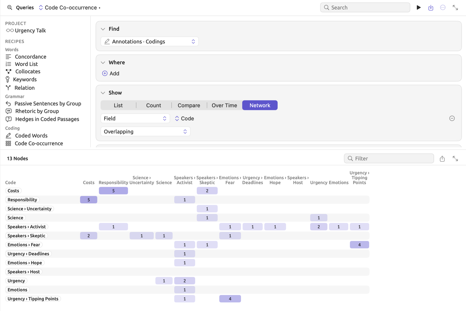
For showing code co-occurrence:
- Under Recipes in the left column of a Queries section, click Code Co-occurrence. The recipe finds Codings, groups them by Code, and links codings that overlap.
To link hits in another way, choose an option in the menu showing Overlapping:
- Overlapping links two hits that overlap each other, i.e., have some characters overlapping.
- In the Same Sentence As links hits that begin in the same sentence as each other, for example codings or words. Only hits in indexed documents are linked. When Find is Sentences, each hit is a sentence of its own, so no hits are linked.
- In the Same Paragraph As links hits that begin in the same paragraph as each other.
- In the Same Turn As links hits that begin in the same speaker turn of a transcript, for example codings. When Find is Speaker Turns, each hit is a turn of its own, so no hits are linked.
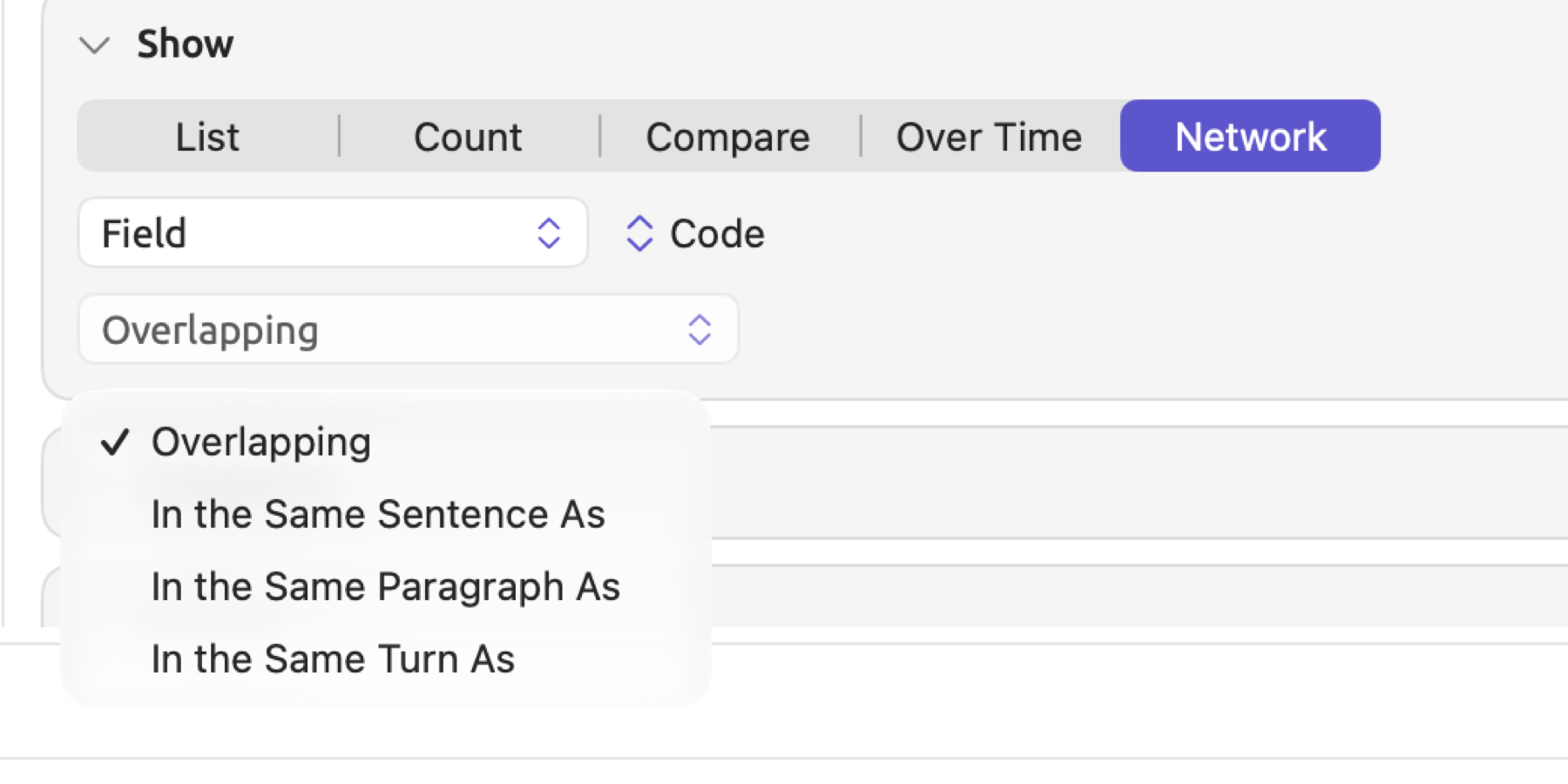
The result is a symmetric table whose rows and columns are all values, with the number of values displayed by the results bar, e.g., 13 Nodes, and whose cells are counts of the pairs of linked hits with those two values. Thus, if the cell with values “Emotions › Fear” and “Urgency › Tipping Points” has 4 entries, 4 overlapping pairs occur, each containing “Fear” and “Tipping Points”. An instance of coding “Fear” overlapping with 3 instances of “Tipping Points” counts for 3 toward this total. Diagonal cells that compare hit values with themselves are always empty because only pairs of hits with different values are counted. Darker cells hold larger counts.
A network has one Group By key. It shows by default the 40 values with the most hits and links no more than the first 2,000 hits per document. For tests of co-occurrence between codes, see Co-occurrences in a document in Chapter 13, Analyzing Codes.
Exporting results
Should you wish to take your results elsewhere, document the process of discovery, or share them, export your results. When there is a result available for a query, the Export button appears at the right of the results bar. In a document’s Query facet, the Export button appears in the facet’s bar at the top instead. Available formats are CSV, Markdown, PNG, and PDF; Copy is also available below them. Except for Copy, choosing each format brings up a save dialog with the query’s name being the default filename.
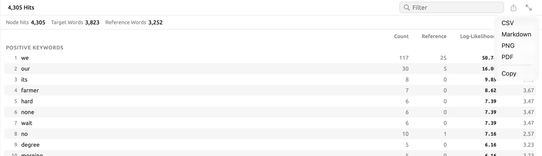
CSV
The CSV format stores results in tabular form which spreadsheet and statistics software can then access. Select the CSV option when you wish to conduct calculations or visualizations yourself. The columns will vary depending on the particular result:
| Result | Columns |
|---|---|
| Concordance or records | The columns of the list |
| One number | Measure, Value, Hits, Documents |
| One Group By key | The key, the measure (or Value for Hits and Documents), Hits, Documents |
| Two Group By keys | Both key names in the first column, then one column for each value of the second key |
| Line chart | The key, Series, the measure (or Value for Hits and Documents), Hits |
| Position in Document | Document, Hits, Size, Positions |
| Collocates | The collocate, Count, Frequency, the score, Log-Likelihood |
| Keywords | The word, Target, Reference, Log-Likelihood, Log Ratio, Direction |
| Network | The key, then one column for each value |
Library units other than Documents export without the Documents column.
Numbers will use digits and a decimal point only, for example 12431.5, regardless of what language your Mac uses. Coverage and Share numbers will be presented as decimals; 0.1296 stands for 13.0%. In Per 10,000 Words, there are two digits past the decimal point. Size refers to the document size used for the calculation of DP, which equals either the document’s word count or, in the cases explained in Where hits fall in each document, its character count. Positions show at what position in each document each hit starts, in terms of fractions between 0 and 1 separated with spaces. Direction indicates whether a particular keyword is positive or negative. If a result contains a test, then the final row will contain the test; for instance, Kruskal-Wallis H, H(2) = 3.429, p = 0.1801, ε² = 0.686.
The file is saved in UTF-8 format, meaning that all kinds of special letters or Chinese characters will pass through unchanged into a spreadsheet application. All cells that are not numbers and start with the signs =, +, -, or @ receive an apostrophe as prefix, ensuring that spreadsheets treat them as text.
Markdown with provenance
A Markdown file captures both the results of a query and how those results were produced. The contents of a Markdown file include:
- Name of the query, which is presented as a heading
- The query itself, as displayed in the Query Text condition
- Scope, the document, set, or project selected for the query
- Documents, number of documents analyzed relative to total documents, as in 12 of 14
- Corpus, the setting in the Options condition
- Measure, whenever the result uses one
- Date, date when the export was performed, along with LemmaLoom Version
- Result
- Test result, whenever available, presented as in the CSV file, such as
Kruskal-Wallis H: H(2) = 3.429, p = 0.1801, ε² = 0.686
A concordance displays as quotations in a sequence, one per hit, with the match in bold and the document name followed by its location underneath. Every other result displays in a Markdown table identical in columns to the CSV file format.
PNG and PDF
PNG and PDF are formats for exporting a snapshot of the results to a slide presentation or hard-copy report. The image has a width of about 900 points, in whichever appearance, light or dark, LemmaLoom is using. Up to 200 rows or hits can be included, and a line at the bottom displays the scope, the number of documents read, and the date. In the picture, a concordance includes only the left context, the match itself, and the right context. A test result is listed underneath its table.
The PNG is rendered at twice the resolution. The PDF is a single page with a height determined by the length of your results; the text and lines remain crisp regardless of zoom level, making it useful for printing.
Copy
Copy creates a tab-delimited representation of the same table as the CSV file on the clipboard. Paste this into a spreadsheet program, or a word processor’s table feature. Additional information on the other exports in LemmaLoom can be found in Chapter 22, Exchanging and Exporting.